When working with large Excel spreadsheets, rows of data can easily blend together, making it difficult to keep track of information accurately. Alternating row colors in Excel — often called banded rows — provides an easy and effective way to improve readability, enhance visual structure, and reduce mistakes in financial reports, inventory lists, or large data summaries.
Excel offers several quick and flexible ways to apply alternate row colors. You can use Conditional Formatting for precise control, Table Styles for instant results, or automate the process across multiple files using Python with Spire.XLS for Python. Each approach has its own advantages depending on how frequently you work with Excel data.
Alternating row colors not only make your data easier to read but also help maintain a clean, professional look across different worksheets. In this guide, you’ll learn how to alternate row colors in Excel step by step—covering both built-in methods and Python automation for advanced users.
Methods Overview
You can explore each method below:
- Alternate Row Colors in Excel by Conditional Formatting
- Apply Built-in Table Styles to Color Every Other Row
- Automate Alternating Excel Row Colors with Python
- Comparison of Methods
Why and How to Alternate Row Colors in Excel
Alternating row colors improves readability, data comparison, and professional presentation. This technique helps your eyes follow each row across columns, reducing the risk of reading errors. Many users rely on manual coloring—selecting every other row and applying a background color—but this approach is inefficient. When you insert or delete rows, the colors no longer align properly.
However, this manual method quickly becomes impractical, especially when rows are inserted or deleted. Fortunately, Excel provides smarter and dynamic approaches that automatically maintain color consistency. Let’s explore how to alternate row colors in Excel using built-in tools before moving on to the automated Python method.
Method 1 – Use Conditional Formatting to Alternate Row Colors
Conditional Formatting is one of Excel’s most flexible features. It lets you apply dynamic styles based on logical rules — making it perfect for automatically alternating row colors without manually adjusting the format each time.
Step 1: Select the Data Range
Highlight the range of cells you want to format, such as A1:D20. The rule will apply only within this selection.
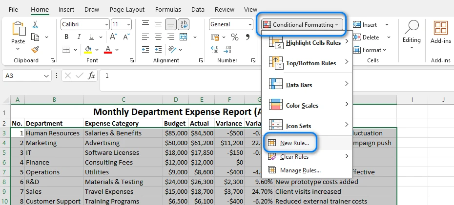
Step 2: Create a Conditional Formatting Rule
Navigate to Home → Conditional Formatting → New Rule
Step 3: Enter the Formula
Choose Use a formula to determine which cells to format. In the formula box, type:
=MOD(ROW(),2)=0
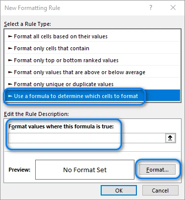
This formula checks whether a row number is even. You can change the “0” to “1” if you want the color pattern to start from the first row instead of the second.
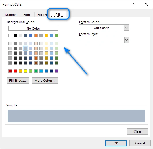
Step 4: Choose a Fill Color
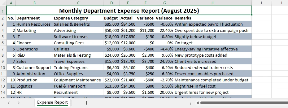
Click Format → Fill, select your preferred background color (a light shade is recommended), and confirm. Once applied, Excel automatically colors every even-numbered row. If you insert new rows, the pattern will update dynamically.
Below is an example of the result:
Tips and Variations
- Use =MOD(ROW(),3)=0 to color every third row instead.
- Combine with text or border formatting for more advanced styling.
- To remove the rule, go to Conditional Formatting → Manage Rules → Delete.
Conditional Formatting offers high flexibility and works perfectly when you need full control over which rows are colored.
Related Article: Apply Conditional Formatting in Excel Using Python
Method 2 – Apply Table Styles for Built-in Alternate Row Colors
If you want a quick, built-in option that requires no formulas, Excel’s Format as Table feature can instantly apply alternate row colors. It’s ideal for users who value speed and prefer minimal setup.
Step 1: Format the Range as a Table
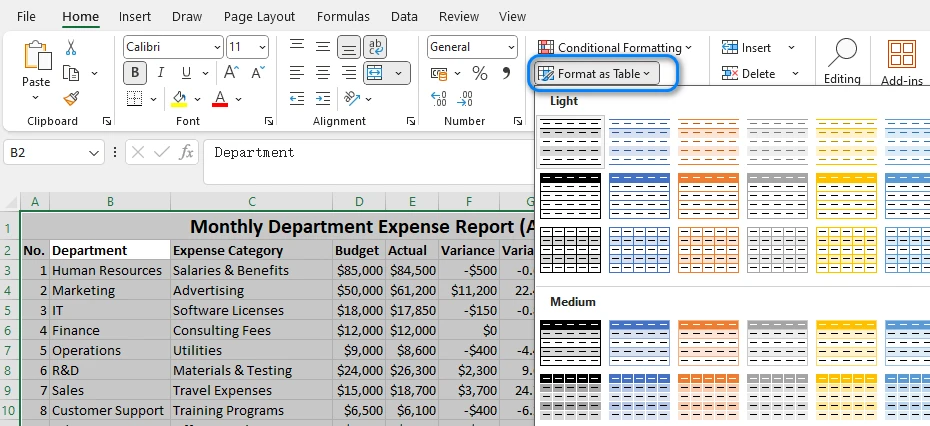
Select your data, then click Home → Format as Table and choose any predefined style. Excel instantly applies banded rows and creates a table structure with sorting and filtering options.
Step 2: Adjust the Table Settings
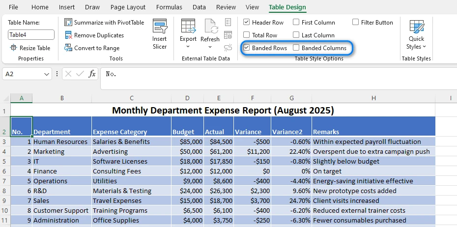
Under the Table Design tab, you can toggle Banded Rows or Banded Columns on or off. You can also customize the color scheme by choosing a different table style.
Step 3: Customize the Table Appearance
You can rename the table, change header colors, or add a Total Row. When new rows are added, the alternating color pattern automatically expands.
Advantages and Limitations
- Quick and professional appearance
- Automatically updates with new data
But:
- Less flexible than Conditional Formatting
- Limited customization of color intervals
For most Excel users, Table Styles are the fastest way to color every other row without formulas. This is the fastest way to apply alternate row color in Excel for quick data formatting.
You may also like: Create or Delete Tables in Excel with Python
Method 3 – Automate Alternating Row Colors in Excel with Python
While Excel’s built-in options work well for single files, they become time-consuming when applied repeatedly. If you frequently handle multiple spreadsheets or need consistent styling across reports, Python automation offers a scalable alternative.
Using Spire.XLS for Python, you can easily control formatting styles, automate row coloring, and even apply conditional logic — saving significant time when processing large or repeated tasks.
Step 1: Install and Import Spire.XLS
Install the package using pip:
pip install spire.xls
Then import it:
from spire.xls import Workbook, Color, ExcelVersion
Step 2: Load and Access the Worksheet
workbook = Workbook()
workbook.LoadFromFile("input.xlsx")
sheet = workbook.Worksheets[0]
This loads your Excel file and accesses the first worksheet.
Step 3: Apply Alternate Row Colors Automatically
for i in range(1, sheet.LastRow):
    if i % 2 == 0:
        style = sheet.Rows.get_Item(i).Style
        style.Color = Color.get_LightGray()
Explanation:
- The loop checks if a row number is even (
i % 2 == 0). - If true, a new style is applied with a light gray background.
- You can customize the color using any supported RGB or theme color.
- For every third or fourth row, adjust the modulus value (e.g.,
i % 3 == 0).
This method can be adapted for different patterns or multiple worksheets within the same workbook.
Step 4: Save the File
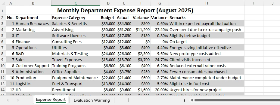
workbook.SaveToFile("output.xlsx", ExcelVersion.Version2016)
The new file will retain all formatting changes, and you can open it directly in Excel. Below is a example of the output file:
Benefits of the Python Method
- Automates repetitive formatting tasks
- Works across multiple sheets or files
- Reduces manual errors
- Integrates seamlessly with other data processing workflows
For large or repetitive tasks, automating with Spire.XLS for Python is a practical way to streamline your workflow and maintain consistent formatting across multiple files. If you want to learn more Python Excel automation skills, check out Spire.XLS for Python tutorials.
Comparison of Methods
| Method | Automation | Customization | Dynamic Updates | Best For |
|---|---|---|---|---|
| Manual Coloring | ❌ | High | ❌ | Quick, one-time edits |
| Conditional Formatting | ✅ | High | ✅ | Flexible formatting |
| Table Style | ✅ | Medium | ✅ | Fast table design |
| Python Automation | ✅ | High | ✅ | Batch or large-scale tasks |
Each approach has its advantages, but automation offers the best efficiency for advanced or repeated Excel formatting.
Frequently Asked Questions About Alternating Row Colors in Excel
Q1: How do I alternate row colors in Excel automatically?
You can use Conditional Formatting with the formula =MOD(ROW(),2)=0 or apply a Table Style to format your data instantly.
Q2: Can I alternate row colors without using a table?
Yes. Conditional Formatting works on any range and updates automatically when you add or remove rows.
Q3: How to color every other row in Excel using Python?
You can automate the process using Spire.XLS for Python, looping through rows and applying a style to even-numbered ones.
Q4: Can I change the color pattern to every 3 rows instead of 2?
Yes. Modify the formula to =MOD(ROW(),3)=0 or change the condition in your Python code (if i % 3 == 0:).
Conclusion
Alternating row colors in Excel is one of the simplest yet most effective ways to make your data easier to read and understand. You can alternate row colors in Excel easily using Conditional Formatting, Table Styles, or Python automation.
For those who work with large datasets or need automation, Spire.XLS for Python makes it easy to apply alternating colors and other formatting tasks programmatically. You can also use Free Spire.XLS for Python for lightweight Excel tasks.
Whichever method you choose, these techniques will help you maintain clarity and consistency in your Excel sheets.