Managing data effectively often requires visual cues to signal completion or updates. Whether you are managing a daily task list, tracking inventory, or auditing financial records, learning how to do strikethrough in Excel is an essential skill for staying organized. Excel doesn't feature a strikethrough button on the default Home ribbon, which can be frustrating for new users. However, by using a specific Excel hotkey for strikethrough or accessing the formatting menu, you can quickly cross out information without deleting the underlying data.
- Strikethrough Text in Excel Cells with Basic Methods
- Adding Strikethrough to Your Quick Access Toolbar
- Strikethrough Using Conditional Formatting
- Programmatic Strikethrough with Free Spire.XLS
- FAQs
How to Strikethrough Text in Excel Cells (Basic Methods)
Mastering the basics is the first step toward spreadsheet efficiency. Most users search for how to strikethrough text in an Excel cell because they need a way to mark items as "done" or "obsolete" while keeping the record visible for future reference.
There are two primary ways to achieve this manually: using fast keyboard commands or navigating through the standard formatting tool. Both methods are effective for formatting either an entire cell or just a specific string of text within a cell.
The Ultimate Shortcut for Strikethrough in Excel
Efficiency is key when handling large datasets. If you find yourself frequently needing to do strikethrough in Excel, memorizing the keyboard shortcut will save you hours of clicking through menus over time.
- For Windows Users: The standard shortcut for strikethrough in Excel is Ctrl + 5. Simply select your cell (or highlight text inside the formula bar) and press these keys simultaneously.
- For Mac Users: The most direct strikethrough shortcut in Excel on Mac is Command + Shift + X. If you prefer a more visual approach, you can press Command + 1 to open the Format Cells dialog, navigate to the Font tab, and manually check the "Strikethrough" box.
Note: These shortcuts are toggles. If you press them a second time on the same cell, the strikethrough effect will be removed immediately.
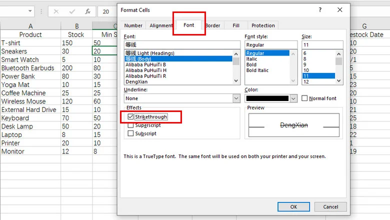
Manual Method: Using the Format Cells Tool
If you aren't a fan of keyboard shortcuts, the classic Format Cells menu offers a visual way to apply styles. This method is often considered the most reliable way to cross out text in Excel because it allows you to preview the font changes before applying them to your spreadsheet.
Step-by-Step Instructions:
- Right-click on the cell or the specific text you wish to format.
- Select Format Cells from the context menu (or press Ctrl + 1).
- Navigate to the Font tab in the popup window.
- Under the Effects section, check the box labeled Strikethrough.
- Click OK to apply the change.
Tip: If you are looking to further polish your cell's appearance, you might also want to learn how to rotate text in Excel to create professional headers.
Advanced: Adding Strikethrough to Your Quick Access Toolbar
For those who perform this action dozens of times a day, even a shortcut might feel repetitive. You can actually customize your workspace to include a dedicated button for this function, making it easier than ever to do strikethrough in Excel with a single click.
Step-by-Step Instructions:
- Click the small drop-down arrow on the Quick Access Toolbar (located at the very top of your Excel window).
- Select More Commands from the list.
- Under "Choose commands from," select All Commands.
- Scroll down to find Strikethrough and click the Add >> button to move it to your toolbar.
- Click OK to save your changes.
Adding these frequently used buttons to your ribbon saves time. Just as you’ve added a strikethrough button, mastering different ways to wrap text will help you keep your headers and data neat with minimal clicks.
Dynamic Strikethrough: Using Conditional Formatting
Sometimes, you want Excel to do the heavy lifting for you. By using conditional formatting, you can set up a rule that automatically applies a strikethrough text in Excel cell style based on the value of another cell.
Step-by-Step Instructions:
- Highlight the cells you want to be automatically crossed out (e.g., task names in Column A).
- Go to the Home tab and click Conditional Formatting > New Rule.
- Select Use a formula to determine which cells to format.
- In the formula box, enter a rule like
=$B2="Done"(assuming Column B contains your status). - Click the Format button, go to the Font tab, and check the Strikethrough box.
- Click OK on both windows to apply the rule.
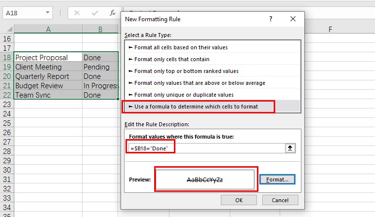
Now, whenever you type "Done" in Column B, the corresponding task in Column A will be instantly struck through. This is the smartest way to strikethrough text in an Excel cell without lifting a finger once the setup is complete.
Programmatic Strikethrough: Using Free Spire.XLS for Python
For developers and data analysts, manual clicking is not an option when dealing with thousands of generated reports. In these cases, using a robust library like Free Spire.XLS allows you to automate how to do strikethrough in Excel through code.
Using Free Spire.XLS, you can programmatically define styles for specific ranges. This is particularly useful for automated financial auditing or generating before and after reports where changes need to be visually highlighted.
from spire.xls import *
from spire.xls.common import *

# Create a Workbook instance and load an Excel file
workbook = Workbook()
workbook.LoadFromFile("/input/sales report.xlsx")

# Get a worksheet
sheet = workbook.Worksheets[0]

# Apply strikethrough to specific cells
sheet.Range["H3"].Style.Font.IsStrikethrough = True
sheet.Range["H10"].Style.Font.IsStrikethrough = True

# Save the modified Excel file
workbook.SaveToFile("/output/Updated_Tasks.xlsx", ExcelVersion.Version2016)
workbook.Dispose()
The preview of the output Excel file:
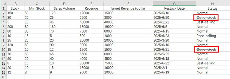
This approach allows you to apply strikethrough formatting programmatically across large datasets, ensuring consistency across enterprise-level documentation without human error.
Furthermore, Free Spire.XLS can be seamlessly combined with conditional formatting logic. For instance, in the inventory file shown above, you can write code to automatically apply a strikethrough to any cell in Column H whenever its value is set to "Out of Stock". This ensures your data remains dynamic and visually intuitive without any manual intervention.
Conclusion
Mastering how to do strikethrough in Excel is a small but powerful way to improve your data visualization and project management. Whether you prefer the speed of a shortcut for strikethrough in Excel, the precision of the Format Cells menu, or the automation power of Free Spire.XLS, there is a solution tailored to your specific workflow. By incorporating these techniques, you can transform a static spreadsheet into a functional, easy-to-read dashboard.
FAQs about Strikethrough in Excel
Q1: What is the shortcut for strikethrough in Excel?
A: Use Ctrl + 5 on Windows or Command + Shift + X on Mac. It’s a toggle, so pressing it again removes the effect.
Q2: How to strikethrough a whole row in Excel?
A: Use Conditional Formatting. Select your range and use a formula like =$B2="Done". The $ ensures the entire row is crossed out based on one cell's value.
Q3: What is the Alt code for strikethrough?
A: There is no direct Alt code, but you can use the sequence Alt > H > 4 on Windows to apply it via the ribbon menu.
Q4: Can I use Ctrl + E for strikethrough?
A: Ctrl + E is for Flash Fill. For strikethrough, you need to use Ctrl + 5.