Comparing columns in Excel is a fundamental, high-value skill for data analysts, accountants, marketers, and all business professionals working with spreadsheets. Whether you’re reconciling financial invoices, scrubbing duplicate customer records, matching inventory SKUs, or validating survey response data, mastering efficient column comparison techniques eliminates hours of manual work.
Yet despite how common this task is, many Excel users rely on slow, error‑prone methods such as scanning row by row, using the filter dropdown repeatedly, or even printing two lists and marking them with a pen. These approaches not only waste time but also increase the risk of overlooking critical mismatches or duplicates.
That’s exactly why this guide exists. You will learn how to compare two columns in Excel using 7 proven methods—from beginner‑friendly visual checks to advanced automation with VBA and Python.
- Why Compare Columns in Excel?
- 1. Conditional Formatting (Highlight Matches/Differences)
- 2. Excel Formula to Compare Two Columns
- 3. Advanced Methods to Compare Columns in Excel
- Excel Column Comparison Method Cheat Sheet
- Frequently Asked Questions
Why Compare Columns in Excel?
Here are the most common real-world use cases to compare Excel columns:
- Data Reconciliation: Verify that two datasets (e.g., a sales report and a payment log) match.
- Duplicate Detection: Find duplicate values across columns (e.g., duplicate customer IDs or email addresses).
- Difference Identification: Spot discrepancies between two versions of the same data.
- Data Validation: Ensure consistency in data entry (e.g., checking that product codes in one column match a master list).
- Merging Datasets: Prepare data for merging by identifying common or unique values across columns.
No matter your use case, Excel has a method tailored to your skill level and data size. We’ll start with the simplest methods (great for beginners) and move to advanced techniques (for power users).
1. Conditional Formatting (Highlight Matches/Differences)
Conditional formatting is the fastest way to visually compare 2 columns in Excel. It highlights matches or differences with colors, making discrepancies easy to spot at a glance.
Best for: Quick visual identification without writing formulas.
How to Use Conditional Formatting:
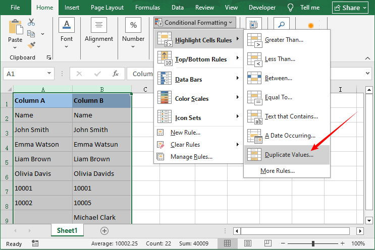
- Select the two columns you want to compare (e.g., Column A and Column B).
- Go to the Home tab in the Excel ribbon.
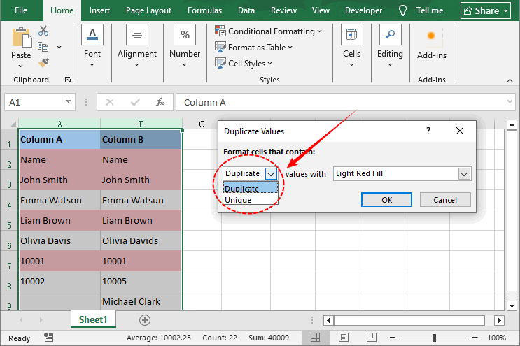
- Click Conditional Formatting → Highlight Cells Rules → Duplicate Values.
- In the pop-up window:
- Choose Duplicate to highlight matching values.
- Choose Unique to highlight differences.
- Select a color scheme and click OK.
Example Result: All matching cells turn light red; differences remain uncolored.
Once you’ve mastered using conditional formatting to highlight matching or unique values between two columns, you can extend the same visual logic to identify data trends—for example, applying data bars to compare sales figures across two regions.
2. Excel Formula to Compare Two Columns
Formula-based methods give you full control over the comparison output. You can return TRUE/FALSE, custom text (“Match” / “Difference”), or even retrieve matching values from another column.
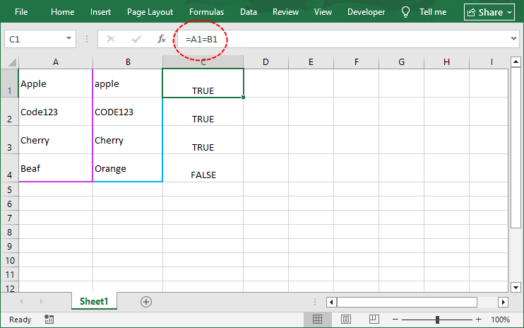
2.1 Equal Operator (=) & EXACT Function
These two methods are the foundation of row‑by‑row comparison. Both compare 2 Excel cells in the same row, but they differ in how they handle letter case. Use the equal operator (=) for case‑insensitive checks, or EXACT when letter case matters.
Case‑Insensitive Equal operator: =A1=B1
- Returns “TRUE” if values match (ignoring case), “FALSE” otherwise.
- Example: "Apple" vs "apple" → TRUE.
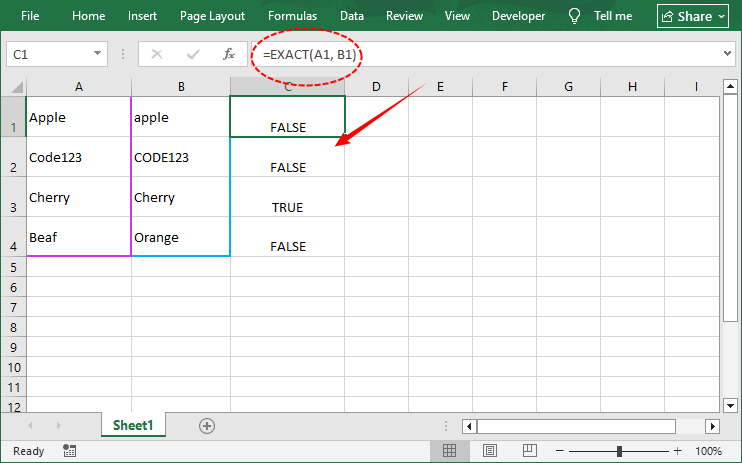
Case-Sensitive EXACT function: =EXACT(A1, B1)
- Returns “TRUE” only if values are identical (including case).
- Example: "Apple" vs "apple" → FALSE.
Related article: How to Remove Duplicate Rows from Excel - 6 Easy Ways
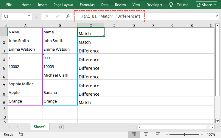
2.2 IF Function (Custom Result Labels)
The IF function lets you replace TRUE/FALSE with custom labels like “Match” or “Mismatch”, making your results easier to interpret. You can even add details about the differences.
Example Formula: =IF(A1=B1, "Match", "Difference")
Variations for different scenarios:
| Scenario | Formula |
|---|---|
| Show only differences (blank if match) | =IF(A1<>B1, "Difference", "") |
| Numeric flag (0 = match, 1 = mismatch) | =IF(A1=B1, 0, 1) |
| Include cell values in message | =IF(A1=B1, "Match", "Mismatch: "&A1&" vs "&B1) |
| Case‑sensitive with custom label | =IF(EXACT(A1,B1), "Exact match", "Case or value differs") |
Why use IF instead of =?
- You can filter on "Match" / "Difference".
- You can combine with other functions to create richer reports.
- Non‑technical users understand words better than TRUE/FALSE.
2.3 VLOOKUP Function (Find Matches Across Columns)
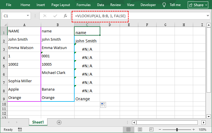
VLOOKUP is the go-to tool for comparing columns with unordered data (e.g., finding a customer ID in Column A that exists in Column B, even if the rows don’t line up).
It searches for a specific value in one column and returns a corresponding value (or an error) if a match is found, making it perfect for finding missing values across columns.
Compare two columns in Excel using VLOOKUP:
- In an empty column (e.g., Column C), enter the formula: =VLOOKUP(A1, B:B, 1, FALSE).
- Breakdown of the formula:
- A1 – the lookup value (what you are searching for).
- B:B – the column to search in (Column B).
- 1 – column index (since B:B has only one column, return that column).
- FALSE – exact match (critical; TRUE would give approximate matches).
- Press Enter. Excel will return the value from Column B if it matches A1, or #N/A if no match is found.
- Drag the fill handle down to apply the formula.
To replace #N/A with a custom label (e.g., "No Match"), wrap the formula in IFERROR: =IFERROR(VLOOKUP(A1, B:B, 1, FALSE), "No Match").
Limitation: VLOOKUP only searches from left to right. To look up values in any direction, use INDEX/MATCH (compatible with all Excel versions) or, if you have Excel 2021 or Microsoft 365, the more intuitive XLOOKUP function.
3. Advanced Methods to Compare Columns in Excel
These methods are for power users working with massive datasets or performing repetitive column comparisons. We cover two automation tools: VBA Macros (Excel-native) and Python (for ultra-scalable data).
3.1 VBA Macro (Built‑in Excel Automation)
VBA (Visual Basic for Applications) allows you to write scripts that run directly inside Excel. Ideal for daily tasks without re‑entering formulas.
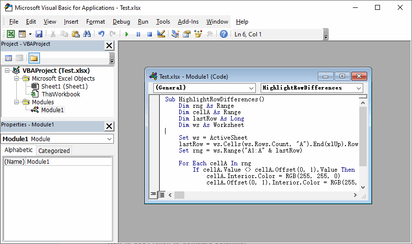
VBA Code to Compare Two Columns in Excel for Differences
Sub HighlightRowDifferences()
    Dim rng As Range
    Dim cellA As Range
    Dim lastRow As Long
    Dim ws As Worksheet

    Set ws = ActiveSheet
    lastRow = ws.Cells(ws.Rows.Count, "A").End(xlUp).Row
    Set rng = ws.Range("A1:A" & lastRow)

    For Each cellA In rng
        If cellA.Value <> cellA.Offset(0, 1).Value Then
            cellA.Interior.Color = RGB(255, 255, 0)      ' Yellow
            cellA.Offset(0, 1).Interior.Color = RGB(255, 255, 0)
        End If
    Next cellA
End Sub
How to use this macro:
- Open your Excel workbook and press Alt + F11 to open the VBA Editor.
- Go to Insert → Module to create a new module.
- Paste the code into the blank module window (customize column/range references as needed).
- Press F5 to run the macro.
Bonus Tip: To make column comparison more accurate, you can use the text to columns feature to split combined cell data (such as names and codes) into separate columns and standardize messy text formats.
3.2 Python with Free Spire.XLS (Scalable & Cross‑Platform)
For developers who need to integrate column comparison into a data pipeline, Python with Free Spire.XLS is the most powerful option. This free library can read, write, and manipulate Excel files without needing Microsoft Excel installed.
Complete Python script to compare two columns:
from spire.xls import *
from spire.xls.common import *

# Create a workbook object
workbook = Workbook()
workbook.LoadFromFile("Test.xlsx")

# Get the first worksheet
sheet = workbook.Worksheets[0]

# Get data range (assume row 1 is header, data starts from row 2)
start_row = 2
end_row = sheet.LastRow

for row in range(start_row, end_row + 1):
    cell_a = sheet.Range[row, 1]
    cell_b = sheet.Range[row, 2]

    # Get values (Handle null values)
    val_a = cell_a.Value if cell_a.Value is not None else ""
    val_b = cell_b.Value if cell_b.Value is not None else ""

    # Compare values
    if val_a == val_b:
        sheet.Range[row, 3].Text = "Match"
    else:
        sheet.Range[row, 3].Text = "Difference"

        # Highlight different cells
        cell_a.Style.Color = Color.get_Yellow()
        cell_b.Style.Color = Color.get_Yellow()

# Save the result file
workbook.SaveToFile("compared.xlsx", ExcelVersion.Version2016)
workbook.Dispose()
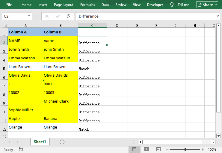
The code loads an Excel file, compares two columns, labels results as “Match” or “Difference”, highlights differences in yellow, and saves a new output file.
After you add a “Match / Difference” column, you can insert a PivotTable to instantly count how many rows matched or differed, transforming a simple column comparison into an intuitive data reporting.
Excel Column Comparison Method Cheat Sheet
Not sure which method to use? Refer to this quick cheat sheet:
| Method | Best For | Skill Level | Pros | Cons |
|---|---|---|---|---|
| Conditional Formatting | Visual checks, small datasets | Beginner | Fast, no formulas, easy to spot differences | No written results, not for large datasets |
| Equal operator & EXACT | Row‑by‑row case‑insensitive or Case‑sensitive comparison | Beginner | Fast and simple formula | Basic output only, no custom labels |
| IF Function | Custom result labels | Intermediate | Easy to interpret, flexible | Requires formula setup |
| VLOOKUP | Unordered data, finding matches | Intermediate | Works with unordered data | Only searches left-to-right |
| VBA Macro | Automation, cross-sheet comparisons | Advanced | Saves time for repetitive tasks | Requires VBA knowledge |
| Python | cross‑platform batch processing, no Excel required | Advanced | Scalable, server‑friendly, and full automation | Requires Python knowledge |
Wrapping up
Comparing two columns in Excel doesn’t have to be a tedious, manual task. The right method depends on your dataset size, skill level, and whether you need visual checks, written results, or automation.
For beginners, start with Conditional Formatting (visual) or the equal operator (quick TRUE/FALSE). For larger datasets or unordered data, use IF or VLOOKUP for custom, readable results. For repetitive tasks or massive datasets, automate the process with a VBA Macro (Excel-native) or Python (scalable).
By mastering these 7 methods, you’ll streamline your data workflow, eliminate manual errors, and turn Excel into a powerful tool for data validation and cleaning.
Frequently Asked Questions
Q1: How do I compare two columns and show differences in a third sheet?
Use the IF function or a VBA macro. For a simple solution: Create a new sheet (e.g., Sheet3), enter =IF(Sheet1!A1=Sheet2!A1, "", "Difference") in the first cell, and drag the fill handle down.
Q2: Can I compare more than two columns at once?
Yes. For row‑wise comparison of three columns (A, B, C):
- Conditional formatting formula: =OR($A1<>$B1, $B1<>$C1) to highlight any mismatch.
- Formula: =IF(AND(A1=B1, B1=C1), "All match", "Mismatch")
- VBA: loop through columns A, B, C and compare each.
- Python: extend the comparison to check all required columns.
Q3: Can I reuse the VBA macro on different workbooks?
Yes. Copy the macro code, and paste it into a new module. Adjust the column letters in the code to match your new data range.
Q4. How can I compare two columns without opening Excel at all?
Use Python with Free Spire.XLS. The script can read the Excel file from disk, perform the comparison, and save the result – all without launching the Excel application. This is ideal for server-side or automated batch processing.