
Spire.XLS for JavaScript (109)
Children categories
Numbers stored in Excel cells often need to be displayed in different formats, such as keeping two decimal places, adding thousands separators, displaying amounts as currency, highlighting negative numbers in red, or showing them as percentages or in scientific notation. Proper number formatting not only makes reports easier to read but also avoids errors caused by manual entry and layout. Spire.XLS for JavaScript completes this directly in the browser based on WebAssembly, and manages input/output files through a virtual file system (VFS), with no backend service required.
Spire.XLS for JavaScript sets number formats through the NumberFormat property of the cell range Range. NumberFormat accepts Excel-standard format code strings. The table below lists the commonly used format code symbols and their meanings:
| Symbol | Description |
|---|---|
0 |
Digit placeholder that always displays a digit, padding with 0 when there are not enough digits |
# |
Digit placeholder that shows only significant digits; extra zeros are not displayed |
? |
Digit placeholder that leaves space for insignificant zeros, used to align decimal points |
. |
Decimal point |
, |
Thousands separator |
% |
Multiplies the number by 100 and displays it as a percentage |
E+ / E- |
Exponent part of scientific notation |
; |
Separates the formats for positive numbers, negative numbers, zeros and text |
[Red] and other color codes |
Sets the display color of the number, e.g. [Red], [Blue], [Green] |
[DBNum1] / [DBNum2] |
Converts numbers to Chinese lowercase / uppercase numerals |
@ |
Text placeholder that displays the number as text |
This article covers three core features:
- Set Decimal Places and Thousands Separator
- Set Currency Format and Highlight Negative Values
- Set Percentage, Scientific Notation and Other Formats
For installation and project configuration, refer to Integrating Spire.XLS for JavaScript in a React Project. The examples below assume Spire.XLS is installed and the WebAssembly module is initialized.
Set Decimal Places and Thousands Separator
When processing amounts, statistics and other data, it is often necessary to keep numbers to a specified number of decimal places, or to add thousands separators for readability. Presenting the same values with the right format codes makes reports easier to scan and avoids manual padding or misplaced commas.
The steps are:
- Load the font file into the VFS for text measurement.
- Create a
Workbookobject and get the first worksheet withWorkbook.Worksheets.get(0). - Use the
Range.Textproperty to write the title, column headers, and the format codes used as description text. - Use the
Range.NumberValueproperty to write the values, and set the corresponding format codes with theRange.NumberFormatproperty. - Use the
Workbook.SaveToFile()method to save the workbook, then release resources withWorkbook.Dispose().
Here is a complete code example showing how to set number formats with different decimal places and thousands separators for cells in React:
function App() {
  const setDecimalPlacesAndThousands = async () => {
    // Get the Spire.XLS WASM module
    const xlsModule = window.wasmModule?.spirexls;

    // Check whether the module is ready
    if (!xlsModule) {
      alert('Spire.Xls is not ready yet');
      return;
    }

    // Load the font into the VFS for text measurement
    await window.spire.FetchFileToVFS('ARIAL.TTF', '/Library/Fonts/', `${process.env.PUBLIC_URL}/font/`);

    // Create a new workbook and get the first worksheet
    const workbook = new xlsModule.Workbook();
    const sheet = workbook.Worksheets.get(0);

    // Write the title and column headers
    sheet.Range.get("B1").Text = "Number Formatting Sample";
    sheet.Range.get("B3").Text = "Format Code";
    sheet.Range.get("C3").Text = "Result";

    // Write the format code in column B, write the value in column C and apply the corresponding number format
    sheet.Range.get("B4").Text = "0";
    sheet.Range.get("C4").NumberValue = 1234.5678;
    sheet.Range.get("C4").NumberFormat = "0";

    sheet.Range.get("B5").Text = "0.00";
    sheet.Range.get("C5").NumberValue = 1234.5678;
    sheet.Range.get("C5").NumberFormat = "0.00";

    sheet.Range.get("B6").Text = "#,##0.00";
    sheet.Range.get("C6").NumberValue = 1234.5678;
    sheet.Range.get("C6").NumberFormat = "#,##0.00";

    // Add a background color to the format-code cells and set the column widths
    sheet.Range.get("B4:B6").Style.KnownColor = xlsModule.ExcelColors.Gray25Percent;
    sheet.SetColumnWidth(2, 26);
    sheet.SetColumnWidth(3, 20);

    // Save the document
    const outputFileName = 'NumberFormat_Decimals_output.xlsx';
    workbook.SaveToFile({ fileName: outputFileName, version: xlsModule.ExcelVersion.Version2010 });

    // Release resources
    workbook.Dispose();

    // Read the converted file from the VFS and trigger a download
    const fileArray = window.dotnetRuntime.Module.FS.readFile(outputFileName);
    const blob = new Blob([fileArray], { type: 'application/vnd.openxmlformats-officedocument.spreadsheetml.sheet' });
    const url = URL.createObjectURL(blob);
    const a = document.createElement('a');
    a.href = url;
    a.download = outputFileName;
    a.click();
    URL.revokeObjectURL(url);
  };

  return (
    <div style={{ textAlign: 'center', height: '300px' }}>
      <h1>Set Decimal Places and Thousands Separator</h1>
      <button onClick={setDecimalPlacesAndThousands}>
        Start
      </button>
    </div>
  );
}

export default App;
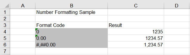
The worksheet after setting decimal places and thousands separator:
Set Currency Format and Highlight Negative Values
In financial reports, amounts are usually displayed in currency format, while negative numbers need to be highlighted so they can be spotted quickly. An Excel number format code can consist of several parts separated by semicolons, so positive and negative values in the same column can be displayed differently, and negative values can be colored on their own.
The steps are:
- Load the font file into the VFS for text measurement.
- Create a
Workbookobject and get the first worksheet withWorkbook.Worksheets.get(0). - Use the
Range.Textproperty to write the title, column headers, and the currency format codes used as description text. - Use the
Range.NumberValueproperty to write the values (including negative numbers), and set the format codes that contain a negative part with theRange.NumberFormatproperty. - Use the
Workbook.SaveToFile()method to save the workbook, then release resources withWorkbook.Dispose().
Here is a complete code example showing how to set a currency format for amounts in React and display negative numbers in red:
function App() {
  const setCurrencyFormat = async () => {
    // Get the Spire.XLS WASM module
    const xlsModule = window.wasmModule?.spirexls;

    // Check whether the module is ready
    if (!xlsModule) {
      alert('Spire.Xls is not ready yet');
      return;
    }

    // Load the font into the VFS for text measurement
    await window.spire.FetchFileToVFS('ARIAL.TTF', '/Library/Fonts/', `${process.env.PUBLIC_URL}/font/`);

    // Create a new workbook and get the first worksheet
    const workbook = new xlsModule.Workbook();
    const sheet = workbook.Worksheets.get(0);

    // Write the title and column headers
    sheet.Range.get("B1").Text = "Number Formatting Sample";
    sheet.Range.get("B3").Text = "Format Code";
    sheet.Range.get("C3").Text = "Result";

    // Set the currency format: two decimal places with a thousands separator
    sheet.Range.get("B4").Text = "$#,##0.00";
    sheet.Range.get("C4").NumberValue = 1234.5678;
    sheet.Range.get("C4").NumberFormat = "$#,##0.00";

    // Negative numbers with a thousands separator displayed in red
    sheet.Range.get("B5").Text = "#,##0.00;[Red]-#,##0.00";
    sheet.Range.get("C5").NumberValue = -1234.5678;
    sheet.Range.get("C5").NumberFormat = "#,##0.00;[Red]-#,##0.00";

    // Negative numbers with two decimal places displayed in red
    sheet.Range.get("B6").Text = "0.00;[Red]-0.00";
    sheet.Range.get("C6").NumberValue = -1234.5678;
    sheet.Range.get("C6").NumberFormat = "0.00;[Red]-0.00";

    // Add a background color to the format-code cells and set the column widths
    sheet.Range.get("B4:B6").Style.KnownColor = xlsModule.ExcelColors.Gray25Percent;
    sheet.SetColumnWidth(2, 26);
    sheet.SetColumnWidth(3, 20);

    // Save the document
    const outputFileName = 'NumberFormat_Currency_output.xlsx';
    workbook.SaveToFile({ fileName: outputFileName, version: xlsModule.ExcelVersion.Version2010 });

    // Release resources
    workbook.Dispose();

    // Read the converted file from the VFS and trigger a download
    const fileArray = window.dotnetRuntime.Module.FS.readFile(outputFileName);
    const blob = new Blob([fileArray], { type: 'application/vnd.openxmlformats-officedocument.spreadsheetml.sheet' });
    const url = URL.createObjectURL(blob);
    const a = document.createElement('a');
    a.href = url;
    a.download = outputFileName;
    a.click();
    URL.revokeObjectURL(url);
  };

  return (
    <div style={{ textAlign: 'center', height: '300px' }}>
      <h1>Set Currency Format and Highlight Negative Values</h1>
      <button onClick={setCurrencyFormat}>
        Start
      </button>
    </div>
  );
}

export default App;
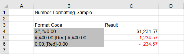
The worksheet after setting the currency format and highlighting negative values:
Set Percentage, Scientific Notation and Other Formats
Besides the common decimal, thousands separator and currency formats, reports often call for percentages, scientific notation and Chinese uppercase amounts. Percentages make proportions easier to compare, scientific notation suits very large or very small numbers, and Chinese uppercase is used on formal financial documents.
The steps are:
- Load the font file into the VFS for text measurement.
- Create a
Workbookobject and get the first worksheet withWorkbook.Worksheets.get(0). - Use the
Range.Textproperty to write the title, column headers, and the format codes used as description text. - Use the
Range.NumberValueproperty to write the values, and set the percentage, scientific notation or Chinese uppercase format codes respectively with theRange.NumberFormatproperty. - Use the
Workbook.SaveToFile()method to save the workbook, then release resources withWorkbook.Dispose().
Here is a complete code example showing how to set percentage, scientific notation and Chinese uppercase formats for cells in React:
function App() {
  const setSpecialNumberFormat = async () => {
    // Get the Spire.XLS WASM module
    const xlsModule = window.wasmModule?.spirexls;

    // Check whether the module is ready
    if (!xlsModule) {
      alert('Spire.Xls is not ready yet');
      return;
    }

    // Load the font into the VFS for text measurement
    await window.spire.FetchFileToVFS('ARIAL.TTF', '/Library/Fonts/', `${process.env.PUBLIC_URL}/font/`);

    // Create a new workbook and get the first worksheet
    const workbook = new xlsModule.Workbook();
    const sheet = workbook.Worksheets.get(0);

    // Write the title and column headers
    sheet.Range.get("B1").Text = "Number Formatting Sample";
    sheet.Range.get("B3").Text = "Format Code";
    sheet.Range.get("C3").Text = "Result";

    // Percentage format: the stored value is multiplied by 100 and a percent sign is shown
    sheet.Range.get("B4").Text = "0.00%";
    sheet.Range.get("C4").NumberValue = 0.1234;
    sheet.Range.get("C4").NumberFormat = "0.00%";

    // Scientific notation format
    sheet.Range.get("B5").Text = "0.00E+00";
    sheet.Range.get("C5").NumberValue = 123456789;
    sheet.Range.get("C5").NumberFormat = "0.00E+00";

    // Chinese uppercase format (uppercase for RMB amounts)
    sheet.Range.get("B6").Text = "[DBNum2][$-804]General";
    sheet.Range.get("C6").NumberValue = 1234567;
    sheet.Range.get("C6").NumberFormat = "[DBNum2][$-804]General";

    // Add a background color to the format-code cells and set the column widths
    sheet.Range.get("B4:B6").Style.KnownColor = xlsModule.ExcelColors.Gray25Percent;
    sheet.SetColumnWidth(2, 26);
    sheet.SetColumnWidth(3, 20);

    // Save the document
    const outputFileName = 'NumberFormat_Special_output.xlsx';
    workbook.SaveToFile({ fileName: outputFileName, version: xlsModule.ExcelVersion.Version2010 });

    // Release resources
    workbook.Dispose();

    // Read the converted file from the VFS and trigger a download
    const fileArray = window.dotnetRuntime.Module.FS.readFile(outputFileName);
    const blob = new Blob([fileArray], { type: 'application/vnd.openxmlformats-officedocument.spreadsheetml.sheet' });
    const url = URL.createObjectURL(blob);
    const a = document.createElement('a');
    a.href = url;
    a.download = outputFileName;
    a.click();
    URL.revokeObjectURL(url);
  };

  return (
    <div style={{ textAlign: 'center', height: '300px' }}>
      <h1>Set Percent, Scientific Notation and Other Formats</h1>
      <button onClick={setSpecialNumberFormat}>
        Start
      </button>
    </div>
  );
}

export default App;
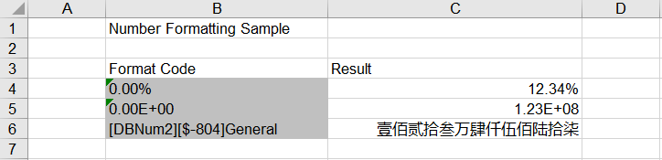
The worksheet after setting percentage, scientific notation and other special formats:
FAQ
The displayed value does not change after setting the number format
Cause: The value written to the cell is actually stored as text, or the data itself is not numeric, so NumberFormat cannot take effect on a number.
Solution: Make sure the value is written with the Range.NumberValue property (rather than a Text or Value string) before setting the NumberFormat, for example:
sheet.Range.get("C4").NumberValue = 1234.5678;
sheet.Range.get("C4").NumberFormat = "0.00";
The value is enlarged after using the percentage format
Cause: Excel displays a percentage format as "stored value × 100". For example, the stored value 12.34 combined with the 0.00% format is displayed as 1234.00%, not 12.34%.
Solution: To display 12.34%, the stored value should be 0.1234. If the original data was entered as a percentage number, divide it by 100 before setting the format.
Negative numbers are not displayed in red
Cause: When a format code contains only one section, positive numbers, negative numbers and zeros all use that section, so [Red] in it affects every value. The color applies only to negative numbers when it is placed in the negative section.
Solution: Split the positive and negative parts with a semicolon and put [Red] in the negative part, for example 0.00;[Red]-0.00.
Obtain a Free License
Spire.XLS for JavaScript offers a 30-day full-featured free trial license with no functional limitations. Apply here to evaluate before purchasing.
When data is split into categories and subcategories, each carrying a value, rows of a table make it hard to see at a glance how much of the whole each category represents. A treemap nests rectangles by hierarchy and sizes each rectangle by its value, so subcategories of the same category sit side by side and their proportions can be compared directly. Turning such data into a treemap, then adding labels and fill colors, produces a chart that can go straight into a report or a shared document. Spire.XLS for JavaScript creates and renders treemap charts in the browser through WebAssembly, with input and output files managed by a virtual file system (VFS) and no backend service required.
This article covers two features:
For installation and project setup, see Integrating Spire.XLS for JavaScript in a React Project. The examples below assume that Spire.XLS is installed and the WebAssembly module is initialized.
Create a Treemap Chart
A treemap uses rectangle area to represent values and the nesting of rectangles to represent hierarchy. To build a usable chart, start with three columns, category, item, and value, then set the chart type to tree map and fix the chart position and title. Once the chart is created, saving it in an Excel workbook lets the chart be opened, edited, or shared in spreadsheet software.
How to create a treemap chart and what it produces:
| Call | Result |
|---|---|
window.spire.FetchFileToVFS |
Loads the font file and the test data file into the VFS |
workbook.LoadFromFile({ fileName }) |
Loads the workbook that holds the two-level data |
workbook.Worksheets.get(0) |
Gets the first worksheet of the workbook |
sheet.Charts.Add() |
Adds a chart object to the worksheet |
chart.ChartType = xlsModule.ExcelChartType.TreeMap |
Sets the chart type to tree map |
chart.DataRange = sheet.Range.get("A2:C11") |
Uses two hierarchy columns and one value column as the chart data |
chart.ChartTitle |
Sets the chart title |
chart.TopRow / chart.BottomRow / chart.LeftColumn / chart.RightColumn |
Sets the position and size of the chart on the worksheet |
workbook.SaveToFile({ fileName }) |
Writes the workbook with the treemap chart into the VFS |
The steps are:
- Load the font file and the Excel test file into the VFS with
window.spire.FetchFileToVFS. - Create a workbook with
new Workbook()and load the test file withworkbook.LoadFromFile. - Get the first worksheet with
workbook.Worksheets.get(0). - Add a chart with
sheet.Charts.Add()and setchart.ChartTypetoxlsModule.ExcelChartType.TreeMap. - Set
chart.DataRangetosheet.Range.get("A2:C11"), where the first two columns are the group and the item and the third column decides the rectangle area. - Set
chart.ChartTitle, then fix the chart position and size throughchart.TopRow,chart.BottomRow,chart.LeftColumn, andchart.RightColumn. - Call
workbook.SaveToFileto writeCreateTreeMap.xlsx, release the workbook withworkbook.Dispose, and read the workbook back from the VFS to trigger the download.
Below is the complete example that creates a treemap chart and saves it in an Excel workbook in React:
function App() {
  const createTreeMap = async () => {
    // Get the Spire.XLS WASM module
    const xlsModule = window.wasmModule?.spirexls;

    // Check that the module is ready
    if (!xlsModule) {
      alert('Spire.Xls is not ready yet');
      return;
    }

    // Load the font and the test data file into the VFS
    await window.spire.FetchFileToVFS('ARIAL.TTF', '/Library/Fonts/', `${process.env.PUBLIC_URL}/font/`);
    const inputFileName = 'TreeMapData.xlsx';
    await window.spire.FetchFileToVFS(inputFileName, '', `${process.env.PUBLIC_URL}data/`);

    // Load the workbook
    const workbook = new xlsModule.Workbook();
    workbook.LoadFromFile({ fileName: inputFileName });

    // Get the first worksheet
    const sheet = workbook.Worksheets.get(0);

    // Add a chart and set its type to tree map
    const chart = sheet.Charts.Add();
    chart.ChartType = xlsModule.ExcelChartType.TreeMap;

    // Set the data range: the first two columns are the group and the item, the third is the value
    chart.DataRange = sheet.Range.get('A2:C11');

    // Set the position and size of the chart
    chart.TopRow = 1;
    chart.BottomRow = 20;
    chart.LeftColumn = 1;
    chart.RightColumn = 12;

    // Set the chart title
    chart.ChartTitle = 'Area by cities';

    // Save the workbook with the tree map chart into the VFS
    const outputFileName = 'CreateTreeMap.xlsx';
    workbook.SaveToFile({ fileName: outputFileName });

    // Dispose of the workbook to release its resources
    workbook.Dispose();

    // Read the result back out of the VFS and trigger the download
    const fileArray = window.dotnetRuntime.Module.FS.readFile(outputFileName);
    const blob = new Blob([fileArray], { type: 'application/vnd.openxmlformats-officedocument.spreadsheetml.sheet' });
    const url = URL.createObjectURL(blob);
    const a = document.createElement('a');
    a.href = url;
    a.download = outputFileName;
    a.click();
    URL.revokeObjectURL(url);
  };

  return (
    <div style={{ textAlign: 'center', height: '300px' }}>
      <h1>Create a Tree Map Chart in React</h1>
      <button id="create-treemap" onClick={createTreeMap}>Create Tree Map</button>
    </div>
  );
}

export default App;
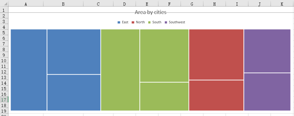
The workbook after creating the treemap chart:
Set Treemap Labels and Fill Colors
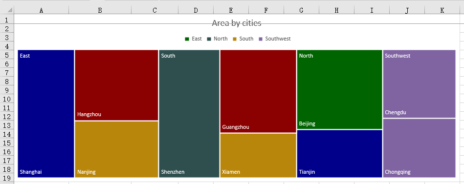
By default, a treemap is rendered without any data labels, so readers can rely only on the legend to tell the groups apart and cannot see which item each area stands for. Rectangles in the same group also share one color, which makes neighboring areas less distinct. Turning on name labels for the rectangles and then assigning darker fill colors in data point order places each item name directly on its area; the white labels stay legible on the dark fills, and both the group structure and the relative sizes become easy to read.
How to set treemap labels and fill colors and what it produces:
| Call | Result |
|---|---|
chart.Series.get(0).DataPoints |
Gets the data point collection, one point per rectangle |
points.get(i).DataFormat.Fill.FillType = xlsModule.ShapeFillType.SolidColor |
Makes that rectangle use a solid fill |
points.get(i).DataFormat.Fill.ForeColor = colors[i % colors.length] |
Assigns a fill color to that rectangle |
chart.Series.get(0).DataPoints.DefaultDataPoint.DataLabels.HasCategoryName = true |
Enables category name labels, so item names appear on the rectangles |
chart.Series.get(0).DataFormat.TreeMapLabelOption = xlsModule.ExcelTreeMapLabelOption.Overlapping |
Overlays item names directly on the rectangles and leaves group names in the group corner |
xlsModule.ExcelTreeMapLabelOption.Banner |
Gives group names a strip at the top of each group and keeps item names inside the rectangles |
xlsModule.ExcelTreeMapLabelOption.None |
Hides every label in the chart |
The steps are:
- Load the test workbook and create the chart as described in the previous section, keeping the data range, position, and title unchanged.
- Get the data points with
chart.Series.get(0).DataPoints, loop over the data rows, and setDataFormat.Fill.FillTypetoxlsModule.ShapeFillType.SolidColorandForeColorto the chosen color for each point. - Set
chart.Series.get(0).DataPoints.DefaultDataPoint.DataLabels.HasCategoryNametotrue. Data labels are off by default on a treemap, so category names appear on the rectangles only after this is enabled. - Set
chart.Series.get(0).DataFormat.TreeMapLabelOptiontoxlsModule.ExcelTreeMapLabelOption.Overlappingso item names are drawn directly on the rectangles; useBannerinstead when group names should take a strip at the top of each group. - Write
TreeMapStyled.xlsxwithworkbook.SaveToFileand trigger the download, then release the workbook withworkbook.Dispose.
Below is the complete example. The chart setup is kept from the previous section so that it runs on its own; the additions are the fill colors and the labels:
function App() {
  const styleTreeMap = async () => {
    // Get the Spire.XLS WASM module
    const xlsModule = window.wasmModule?.spirexls;

    // Check that the module is ready
    if (!xlsModule) {
      alert('Spire.Xls is not ready yet');
      return;
    }

    // Load the font and the test data file into the VFS
    await window.spire.FetchFileToVFS('ARIAL.TTF', '/Library/Fonts/', `${process.env.PUBLIC_URL}/font/`);
    const inputFileName = 'TreeMapData.xlsx';
    await window.spire.FetchFileToVFS(inputFileName, '', `${process.env.PUBLIC_URL}data/`);

    // Load the workbook
    const workbook = new xlsModule.Workbook();
    workbook.LoadFromFile({ fileName: inputFileName });

    // Get the first worksheet
    const sheet = workbook.Worksheets.get(0);

    // Add a tree map chart and set its data range
    const chart = sheet.Charts.Add();
    chart.ChartType = xlsModule.ExcelChartType.TreeMap;
    chart.DataRange = sheet.Range.get('A2:C11');
    chart.TopRow = 1;
    chart.BottomRow = 20;
    chart.LeftColumn = 1;
    chart.RightColumn = 12;
    chart.ChartTitle = 'Area by cities';

    // Prepare the fill colors used in the loop
    const colors = [
      xlsModule.Color.get_DarkGreen(),
      xlsModule.Color.get_DarkBlue(),
      xlsModule.Color.get_DarkGoldenrod(),
      xlsModule.Color.get_DarkRed(),
      xlsModule.Color.get_DarkSlateGray(),
    ];

    // Set the fill color of every rectangle in data point order (10 data rows)
    const points = chart.Series.get(0).DataPoints;
    for (let i = 0; i < 10; i++) {
      points.get(i).DataFormat.Fill.FillType = xlsModule.ShapeFillType.SolidColor;
      points.get(i).DataFormat.Fill.ForeColor = colors[i % colors.length];
    }

    // Enable category name labels and overlay the item names on the rectangles
    chart.Series.get(0).DataPoints.DefaultDataPoint.DataLabels.HasCategoryName = true;
    chart.Series.get(0).DataFormat.TreeMapLabelOption = xlsModule.ExcelTreeMapLabelOption.Overlapping;

    // Save the workbook with the tree map chart into the VFS
    const outputFileName = 'TreeMapStyled.xlsx';
    workbook.SaveToFile({ fileName: outputFileName });

    // Dispose of the workbook to release its resources
    workbook.Dispose();

    // Read the result back out of the VFS and trigger the download
    const fileArray = window.dotnetRuntime.Module.FS.readFile(outputFileName);
    const blob = new Blob([fileArray], { type: 'application/vnd.openxmlformats-officedocument.spreadsheetml.sheet' });
    const url = URL.createObjectURL(blob);
    const a = document.createElement('a');
    a.href = url;
    a.download = outputFileName;
    a.click();
    URL.revokeObjectURL(url);
  };

  return (
    <div style={{ textAlign: 'center', height: '300px' }}>
      <h1>Create a Tree Map Chart in React</h1>
      <button id="style-treemap" onClick={styleTreeMap}>Set Labels and Fill Colors</button>
    </div>
  );
}

export default App;
The workbook after setting treemap labels and fill colors:
FAQ
Treemap labels do not appear
Cause: Data labels are off by default on a treemap, so no names are drawn on the rectangles. TreeMapLabelOption only controls how labels are laid out, and setting it alone does not make labels visible.
Solution: Set DataLabels.HasCategoryName on the data points to true first, then set TreeMapLabelOption: use Overlapping to draw item names directly on the rectangles, or Banner to give group names a strip at the top of each group. For example:
chart.Series.get(0).DataPoints.DefaultDataPoint.DataLabels.HasCategoryName = true;
chart.Series.get(0).DataFormat.TreeMapLabelOption = xlsModule.ExcelTreeMapLabelOption.Overlapping;
How can the position and size of a treemap be adjusted
Cause: The position of a chart is controlled by TopRow, BottomRow, LeftColumn, and RightColumn, which mark the first and last row and column the chart covers.
Solution: Adjust these four properties before saving the workbook. Larger values widen the range of rows and columns the chart covers, so the chart takes up more space on the worksheet.
How should the data for a treemap be arranged
Cause: A treemap reads hierarchy and values by column, so the order of the columns determines how groups, items, and areas correspond to one another.
Solution: Arrange the data in three columns: the first for the category, the second for the item, and the third for the value, and keep the value column numeric. Start chart.DataRange at the first data row, for example sheet.Range.get("A2:C11"), so the header row is not included.
Get a Free License
Spire.XLS for JavaScript offers a 30-day full-featured free trial license with no functional limitations. Apply here to evaluate before purchasing.
In everyday data analysis, a scatter chart is an intuitive tool for examining the relationship between two numeric variables — for example, exploring the correlation between product price and sales, or income and spending. With a scatter chart, you can quickly spot how data points are distributed and any potential relationships. Spire.XLS for JavaScript creates scatter charts directly in the browser based on WebAssembly, and manages input/output files through a virtual file system (VFS), with no backend service required.
This article covers two core features:
For installation and project configuration, refer to Integrating Spire.XLS for JavaScript in a React Project. The examples below assume Spire.XLS is installed and the WebAssembly module is initialized.
Create a Basic Scatter Chart
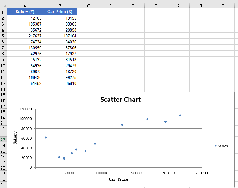
A scatter chart places two sets of numeric values on the horizontal and vertical axes, using the position of each point to show how the two variables correspond. Compared with reading a table, it makes clusters, gaps and upward or downward relationships easier to see. Mapping the source data onto the chart and fixing its position on the worksheet is all it takes to start examining that relationship.
Creating a basic scatter chart:
| Syntax | Result |
|---|---|
workbook.LoadFromFile(...) |
Loads the workbook that contains the source data |
sheet.Charts.Add({ chartType: xlsModule.ExcelChartType.ScatterMarkers }) |
Adds a scatter chart with data markers to the worksheet |
chart.DataRange = sheet.Range.get("B2:B13") |
Sets the data range used by the chart |
chart.Series.get(0).CategoryLabels = sheet.Range.get("A2:A13") |
Uses column A for the horizontal axis |
chart.Series.get(0).Values = sheet.Range.get("B2:B13") |
Uses column B for the vertical axis |
chart.LeftColumn / TopRow / RightColumn / BottomRow |
Positions the chart on the worksheet |
chart.ChartTitle, PrimaryCategoryAxis.Title, PrimaryValueAxis.Title |
Sets the chart title and the axis titles |
workbook.SaveToFile(...) |
Saves the workbook with the scatter chart to the VFS |
The steps are:
- Load the font file and the source data file into the VFS.
- Create a
Workbookobject, load the Excel document withWorkbook.LoadFromFile(), and get the first worksheet withWorkbook.Worksheets.get(0). - Use the
Worksheets.Charts.Add()method with theScatterMarkerschart type to add a scatter chart. - Set the chart's
DataRangeandSeriesDataFromRange, and specify the horizontal and vertical axis data withSeries.get(0).CategoryLabelsandSeries.get(0).Values. - Set the chart position with the
LeftColumn,TopRow,RightColumnandBottomRowproperties. - Set the chart title with the
ChartTitleproperty, and set the X-axis and Y-axis titles with thePrimaryCategoryAxis.TitleandPrimaryValueAxis.Titleproperties. - Use the
Workbook.SaveToFile()method to save the document, then release resources withDispose().
Here is a complete code example showing how to create a basic scatter chart in React:
function App() {
  const createScatterChart = async () => {
    // Get the Spire.XLS WASM module
    const xlsModule = window.wasmModule?.spirexls;

    // Check whether the module is ready
    if (!xlsModule) {
      alert('Spire.Xls is not ready yet');
      return;
    }

    // Load the font and Excel file into the VFS
    await window.spire.FetchFileToVFS('ARIAL.TTF', '/Library/Fonts/', `${process.env.PUBLIC_URL}/font/`);
    const inputFileName = 'ScatterChartData.xlsx';
    await window.spire.FetchFileToVFS(inputFileName, '', `${process.env.PUBLIC_URL}data/`);

    // Load the workbook
    const workbook = new xlsModule.Workbook();
    workbook.LoadFromFile({ fileName: inputFileName });

    // Get the first worksheet
    const sheet = workbook.Worksheets.get(0);

    // Add a scatter chart with data markers
    let chart = sheet.Charts.Add({ chartType: xlsModule.ExcelChartType.ScatterMarkers });

    // Set the chart's data range
    chart.DataRange = sheet.Range.get("B2:B13");
    chart.SeriesDataFromRange = false;

    // Set the series data: column A for the X-axis and column B for the Y-axis
    chart.Series.get(0).CategoryLabels = sheet.Range.get("A2:A13");
    chart.Series.get(0).Values = sheet.Range.get("B2:B13");

    // Set the position of the chart
    chart.LeftColumn = 1;
    chart.TopRow = 15;
    chart.RightColumn = 10;
    chart.BottomRow = 32;

    // Set the chart title
    chart.ChartTitle = "Scatter Chart";

    // Set the X-axis and Y-axis titles
    chart.PrimaryCategoryAxis.Title = "Car Price";
    chart.PrimaryValueAxis.Title = "Salary";

    // Save the document
    const outputFileName = 'CreateScatterChart_output.xlsx';
    workbook.SaveToFile({ fileName: outputFileName });

    // Release resources
    workbook.Dispose();

    // Read the converted file from the VFS and trigger a download
    const fileArray = window.dotnetRuntime.Module.FS.readFile(outputFileName);
    const blob = new Blob([fileArray], { type: 'application/vnd.openxmlformats-officedocument.spreadsheetml.sheet' });
    const url = URL.createObjectURL(blob);
    const a = document.createElement('a');
    a.href = url;
    a.download = outputFileName;
    a.click();
    URL.revokeObjectURL(url);
  };

  return (
    <div style={{ textAlign: 'center', height: '300px' }}>
      <h1>Create Scatter Chart</h1>
      <button onClick={createScatterChart}>
        Start
      </button>
    </div>
  );
}

export default App;
The chart after creating a basic scatter chart:
Add a Trend Line to the Scatter Chart
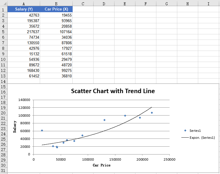
A trend line adds a fitted curve on top of the scatter points to summarize the overall direction of the data. The more scattered the points are, the more useful the trend line becomes for judging whether the variables rise, fall or stay roughly flat together. Adding an exponential trend line to the chart's data series records that trend in the workbook.
Adding a trend line to the scatter chart:
| Syntax | Result |
|---|---|
sheet.Charts.Add({ chartType: xlsModule.ExcelChartType.ScatterMarkers }) |
Adds a scatter chart with data markers |
chart.Series.get(0).TrendLines.Add({ type: xlsModule.TrendLineType.Exponential }) |
Adds an exponential trend line to the first series |
workbook.SaveToFile(...) |
Saves the workbook with the trend line to the VFS |
The steps are:
- Load the font file and the source data file into the VFS.
- Create a
Workbookobject, load the Excel document withLoadFromFile(), and get the first worksheet withWorkbook.Worksheets.get(0). - Use the
Worksheets.Charts.Add()method to add a scatter chart, and setDataRange,CategoryLabelsandValues. - Set the chart title with the
ChartTitleproperty, and set the X-axis and Y-axis titles with the axis title properties. - Use the
Series.get(0).TrendLines.Add()method to add an exponential trend line to the first data series. - Use the
Workbook.SaveToFile()method to save the document, then release resources withDispose().
Here is a complete code example showing how to add an exponential trend line to a scatter chart in React:
function App() {
  const addTrendLine = async () => {
    // Get the Spire.XLS WASM module
    const xlsModule = window.wasmModule?.spirexls;

    // Check whether the module is ready
    if (!xlsModule) {
      alert('Spire.Xls is not ready yet');
      return;
    }

    // Load the font and Excel file into the VFS
    await window.spire.FetchFileToVFS('ARIAL.TTF', '/Library/Fonts/', `${process.env.PUBLIC_URL}/font/`);
    const inputFileName = 'ScatterChartData.xlsx';
    await window.spire.FetchFileToVFS(inputFileName, '', `${process.env.PUBLIC_URL}data/`);

    // Load the workbook
    const workbook = new xlsModule.Workbook();
    workbook.LoadFromFile({ fileName: inputFileName });

    // Get the first worksheet
    const sheet = workbook.Worksheets.get(0);

    // Add a scatter chart
    let chart = sheet.Charts.Add({ chartType: xlsModule.ExcelChartType.ScatterMarkers });
    chart.DataRange = sheet.Range.get("B2:B13");
    chart.SeriesDataFromRange = false;
    chart.Series.get(0).CategoryLabels = sheet.Range.get("A2:A13");
    chart.Series.get(0).Values = sheet.Range.get("B2:B13");

    // Set the position of the chart
    chart.LeftColumn = 1;
    chart.TopRow = 15;
    chart.RightColumn = 10;
    chart.BottomRow = 32;

    // Set the chart title
    chart.ChartTitle = "Scatter Chart with Trend Line";

    // Set the X-axis and Y-axis titles
    chart.PrimaryCategoryAxis.Title = "Car Price";
    chart.PrimaryValueAxis.Title = "Salary";

    // Add an exponential trend line to the first data series
    chart.Series.get(0).TrendLines.Add({ type: xlsModule.TrendLineType.Exponential });

    // Save the document
    const outputFileName = 'ScatterChartTrendLine_output.xlsx';
    workbook.SaveToFile({ fileName: outputFileName });

    // Release resources
    workbook.Dispose();

    // Read the converted file from the VFS and trigger a download
    const fileArray = window.dotnetRuntime.Module.FS.readFile(outputFileName);
    const blob = new Blob([fileArray], { type: 'application/vnd.openxmlformats-officedocument.spreadsheetml.sheet' });
    const url = URL.createObjectURL(blob);
    const a = document.createElement('a');
    a.href = url;
    a.download = outputFileName;
    a.click();
    URL.revokeObjectURL(url);
  };

  return (
    <div style={{ textAlign: 'center', height: '300px' }}>
      <h1>Add Trend Line to Scatter Chart</h1>
      <button onClick={addTrendLine}>
        Start
      </button>
    </div>
  );
}

export default App;
The scatter chart after adding a trend line:
FAQ
Data points are all clustered at the bottom-left of the axes
Cause: The data range set for the chart includes the header row or empty cells. These non-numeric contents are treated as zero or ignored, so all data points cluster at the bottom-left of the axes.
Solution: Make sure the chart data range starts from the data rows (for example sheet.Range.get("A2:A13")), and that CategoryLabels and Values point to the same row range so the X and Y values correspond one-to-one.
Adding an exponential trend line fails
Cause: An exponential trend line requires all data values to be positive. When the data contains zero or negative values, the exponential regression fit cannot be completed, and the trend line may fail to be added or may not be displayed.
Solution: Check whether the data contains zero or negative values. If necessary, use a trend line type that fits the current data, such as linear (Linear) or polynomial (Polynomial).
How do the horizontal and vertical axis values correspond?
Cause: A scatter chart takes the horizontal axis from CategoryLabels and the vertical axis from Values. If the two ranges cover different rows or start at different rows, the points are paired incorrectly and may even fall outside the plot area.
Solution: Point CategoryLabels and Values at the same row range, for example rows 2 through 13, and change only the column. Each horizontal value then has a matching vertical value.
Obtain a Free License
Spire.XLS for JavaScript offers a 30-day full-featured free trial license with no functional limitations. Apply here to evaluate before purchasing.
The header and footer in Excel are text or images placed at the top and bottom of every printed page. The text or images in the header and footer can display basic information about the page or document, such as the file name, company logo, page number, date and time. Spire.XLS for JavaScript completes this directly in the browser based on WebAssembly, managing input/output files through a virtual file system (VFS), with no backend service required.
The PageSetup class provided by Spire.XLS for JavaScript can configure the page of an Excel workbook, including setting the header and footer. The LeftHeader, CenterHeader, RightHeader, LeftFooter, CenterFooter, RightFooter properties in this class add content to the left, center and right of the header or footer. To add fields to the header or footer or to set the text format of the header and footer, you can use the format codes listed in the table below.
| Code | Description |
|---|---|
&P |
Current page number |
&N |
Total number of pages |
&D |
Current date |
&T |
Current time |
&G |
Picture |
&A |
The worksheet name |
&F |
The file name |
&B |
Bold text |
&I |
Italic text |
&U |
Underline text |
&"Font Name" |
The font name, e.g. &"Arial" |
& + Integer |
The font size, e.g. &12 |
&K + 16-digit color code |
The font color, e.g. &KFF0000 |
This article introduces two core features:
For installation and project configuration, refer to Integrating Spire.XLS for JavaScript in a React Project. The examples below assume Spire.XLS is installed and the WebAssembly module is initialized.
Add an Image and Formatted Text to the Header
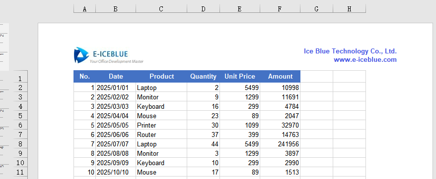
The header sits at the top of every page and is a natural place for a company logo, a document name or other fixed information. Putting the image on the left and text with its own font and color on the right gives every printed or previewed page the same identification without adding it page by page.
Adding an image and formatted text to the header:
| Syntax | Result |
|---|---|
new xlsModule.Stream(imgFileName) |
Reads the image stream from the VFS |
sheet.PageSetup.LeftHeaderImage = image |
Sets the image as the left header image |
sheet.PageSetup.LeftHeader = "&G" |
Displays the image in the left header |
sheet.PageSetup.RightHeader = "&\"Arial\"&B&10&K4253E2..." |
Writes text with the specified font, bold, size and color in the right header |
sheet.ViewMode = xlsModule.ViewMode.Layout |
Switches to Page Layout view for previewing |
workbook.SaveToFile(...) |
Saves the workbook with the header to the VFS |
The steps are:
- Load the font, Excel file and image into the VFS.
- Create a
Workbookobject, load the Excel file withLoadFromFile(), and get the first worksheet withWorkbook.Worksheets.get(0). - Use
Streamto load the image, and set it as the image source of the left header through thePageSetup.LeftHeaderImageproperty. - Use the
PageSetup.LeftHeaderproperty to display the image in the left header. - Use the
PageSetup.RightHeaderproperty to insert formatted text in the right header. - Switch the worksheet to Page Layout view with
ViewMode.Layoutto preview the header. - Use the
Workbook.SaveToFile()method to save the workbook, then release resources withWorkbook.Dispose().
Here is a complete code example showing how to add an image and formatted text to the header of a worksheet in React:
function App() {
  const addImageAndTextToHeader = async () => {
    // Get the Spire.XLS WASM module
    const xlsModule = window.wasmModule?.spirexls;

    // Check whether the module is ready
    if (!xlsModule) {
      alert('Spire.Xls is not ready yet');
      return;
    }

    // Load the font, Excel file and image into the VFS
    await window.spire.FetchFileToVFS('ARIAL.TTF', '/Library/Fonts/', `${process.env.PUBLIC_URL}/font/`);
    const inputFileName = 'HeaderFooter.xlsx';
    await window.spire.FetchFileToVFS(inputFileName, '', `${process.env.PUBLIC_URL}data/`);
    const imgFileName = 'logo.png';
    await window.spire.FetchFileToVFS(imgFileName, '', `${process.env.PUBLIC_URL}data/`);

    // Load the workbook
    const workbook = new xlsModule.Workbook();
    workbook.LoadFromFile({ fileName: inputFileName });

    // Get the first worksheet
    const sheet = workbook.Worksheets.get(0);

    // Load the image and set it as the image source of the left header
    const image = new xlsModule.Stream(imgFileName);
    sheet.PageSetup.LeftHeaderImage = image;
    sheet.PageSetup.LeftHeader = "&G";

    // Add formatted text to the right header
    sheet.PageSetup.RightHeader = "&\"Arial\"&B&10&K4253E2Ice Blue Technology Co., Ltd.  \n www.e-iceblue.com";

    // Switch to Page Layout view to preview the header and footer
    sheet.ViewMode = xlsModule.ViewMode.Layout;

    // Save the document
    const outputFileName = 'HeaderImageAndText_output.xlsx';
    workbook.SaveToFile({ fileName: outputFileName, version: xlsModule.ExcelVersion.Version2010 });

    // Release resources
    workbook.Dispose();

    // Read the converted file from the VFS and trigger a download
    const fileArray = window.dotnetRuntime.Module.FS.readFile(outputFileName);
    const blob = new Blob([fileArray], { type: 'application/vnd.openxmlformats-officedocument.spreadsheetml.sheet' });
    const url = URL.createObjectURL(blob);
    const a = document.createElement('a');
    a.href = url;
    a.download = outputFileName;
    a.click();
    URL.revokeObjectURL(url);
  };

  return (
    <div style={{ textAlign: 'center', height: '300px' }}>
      <h1>Add Image and Formatted Text to Header</h1>
      <button onClick={addImageAndTextToHeader}>
        Start
      </button>
    </div>
  );
}

export default App;
The worksheet after adding an image and formatted text to the header:
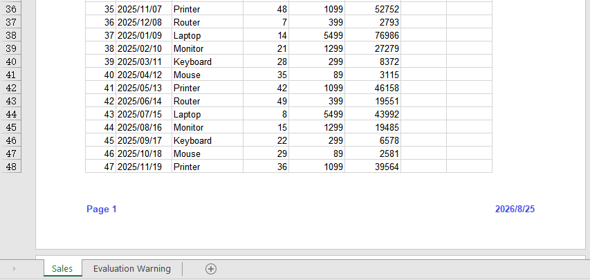
Add the Current Date and Page Number to the Footer
The footer sits at the bottom of every page and is commonly used for page numbers and dates. Both update automatically as pages are printed, so there is no need to maintain them in the sheet body; placing them on the left and right also helps readers find their position when paging through a report.
Adding the current date and page number to the footer:
| Syntax | Result |
|---|---|
sheet.PageSetup.LeftFooter = "...&P..." |
Shows the current page number in the left footer |
sheet.PageSetup.RightFooter = "...&D" |
Shows the current date in the right footer |
sheet.ViewMode = xlsModule.ViewMode.Layout |
Switches to Page Layout view for previewing |
workbook.SaveToFile(...) |
Saves the workbook with the footer to the VFS |
The steps are:
- Load the font and Excel file into the VFS.
- Create a
Workbookobject, load the Excel file withLoadFromFile(), and get the first worksheet withWorkbook.Worksheets.get(0). - Use the
PageSetup.LeftFooterproperty to add a formatted page number to the left footer, customizing its format as you like. - Use the
PageSetup.RightFooterproperty to add the current date to the right footer, and change the appearance of the date text as needed. - Switch the worksheet to Page Layout view with
ViewMode.Layoutto preview the footer. - Use the
Workbook.SaveToFile()method to save the workbook, then release resources withWorkbook.Dispose().
Here is a complete code example showing how to add the current date and page number to the footer of a worksheet in React:
function App() {
  const addDateAndPageNumberToFooter = async () => {
    // Get the Spire.XLS WASM module
    const xlsModule = window.wasmModule?.spirexls;

    // Check whether the module is ready
    if (!xlsModule) {
      alert('Spire.Xls is not ready yet');
      return;
    }

    // Load the font and Excel file into the VFS
    await window.spire.FetchFileToVFS('ARIAL.TTF', '/Library/Fonts/', `${process.env.PUBLIC_URL}/font/`);
    const inputFileName = 'HeaderFooter.xlsx';
    await window.spire.FetchFileToVFS(inputFileName, '', `${process.env.PUBLIC_URL}data/`);

    // Load the workbook
    const workbook = new xlsModule.Workbook();
    workbook.LoadFromFile({ fileName: inputFileName });

    // Get the first worksheet
    const sheet = workbook.Worksheets.get(0);

    // Add the page number to the left footer; &P represents the current page number
    sheet.PageSetup.LeftFooter = "&\"Arial\"&B&10&K4253E2Page &P";

    // Add the current date to the right footer; &D represents the current date
    sheet.PageSetup.RightFooter = "&\"Arial\"&B&10&K4253E2&D";

    // Switch to Page Layout view to preview the header and footer
    sheet.ViewMode = xlsModule.ViewMode.Layout;

    // Save the document
    const outputFileName = 'FooterDatePageNumber_output.xlsx';
    workbook.SaveToFile({ fileName: outputFileName, version: xlsModule.ExcelVersion.Version2010 });

    // Release resources
    workbook.Dispose();

    // Read the converted file from the VFS and trigger a download
    const fileArray = window.dotnetRuntime.Module.FS.readFile(outputFileName);
    const blob = new Blob([fileArray], { type: 'application/vnd.openxmlformats-officedocument.spreadsheetml.sheet' });
    const url = URL.createObjectURL(blob);
    const a = document.createElement('a');
    a.href = url;
    a.download = outputFileName;
    a.click();
    URL.revokeObjectURL(url);
  };

  return (
    <div style={{ textAlign: 'center', height: '300px' }}>
      <h1>Add Current Date and Page Number to Footer</h1>
      <button onClick={addDateAndPageNumberToFooter}>
        Start
      </button>
    </div>
  );
}

export default App;
The worksheet after adding the current date and page number to the footer:
FAQ
Headers and footers are not visible in Excel
Cause: An Excel worksheet is in Normal view by default, and headers and footers are only displayed in Page Layout view or when printing.
Solution: Switch the worksheet to Page Layout view in code with sheet.ViewMode = xlsModule.ViewMode.Layout;, or switch to the "Page Layout" view manually in Excel.
The picture in the header is not displayed
Cause: Only the image source (such as LeftHeaderImage) was set, but the &G placeholder was not used in the corresponding header text, or the image file was not loaded into the VFS correctly.
Solution: Make sure the image has been loaded into the VFS with FetchFileToVFS() and add &G to the header string, for example sheet.PageSetup.LeftHeader = "&G";.
How can the current page number and total page count appear together?
Cause: The footer used only the &P field, so it shows the current page number without any information about the total number of pages.
Solution: Put both &P and &N in the footer string, for example sheet.PageSetup.LeftFooter = "&P / &N";. When printing or previewing, the two fields are replaced with the current page number and the total page count respectively.
Obtain a Free License
Spire.XLS for JavaScript offers a 30-day full-featured free trial license with no functional limitations. Apply here to evaluate before purchasing.
Add and Remove Watermarks in Excel with JavaScript in React
2026-10-23 08:49:10 Written by liu taliaExcel does not have a built-in watermark feature, but in scenarios such as contracts, reports, and internal documents, we often need to mark files with identifiers like "Confidential" or "Sample" to prevent information from being copied and distributed at will. Spire.XLS for JavaScript processes Excel documents directly in the browser based on WebAssembly, and manages input and output files through a virtual file system (VFS), with no backend service required. With the header image feature, you can easily add and remove watermarks in worksheets.
This article covers two core features:
For installation and project configuration, refer to Integrating Spire.XLS for JavaScript in a React Project. The examples below assume Spire.XLS is installed and the WebAssembly module is initialized.
Add a Watermark to an Excel Worksheet
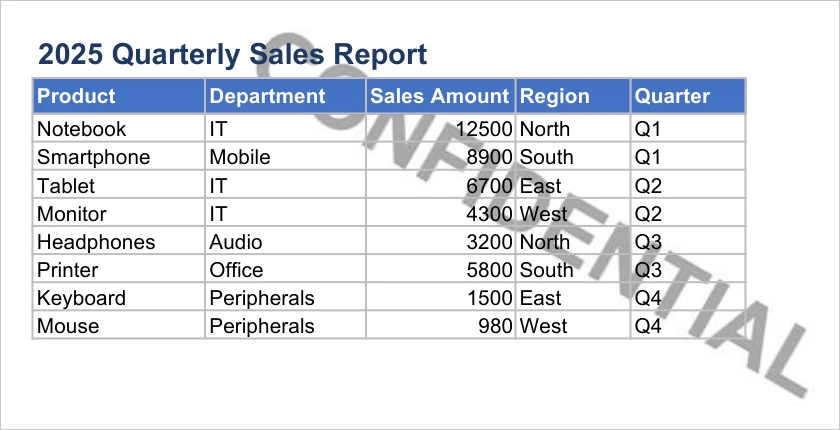
Excel does not have a built-in watermark feature, yet contracts, reports and internal documents often need to mark their origin or scope of use. A watermark lays pale text across the center of the page, leaving the body readable while signaling what the document is for. Drawing the watermark as an image the size of the page and placing it in the header makes it appear on every page.
Adding a watermark to an Excel worksheet:
| Syntax | Result |
|---|---|
sheet.PageSetup.PageWidth / PageHeight |
Gets the page size used to draw a matching watermark image |
watermarkCanvas.toBlob(...) and FS.writeFile(...) |
Creates the watermark image and writes it to the VFS |
new xlsModule.Stream(imgFileName) |
Reads the watermark image stream from the VFS |
sheet.PageSetup.LeftHeaderImage = watermark |
Sets the watermark image as the left header image |
sheet.PageSetup.LeftHeader = "&G" |
Displays the image in the header |
sheet.ViewMode = xlsModule.ViewMode.Layout |
Switches to Page Layout view for previewing |
workbook.SaveToFile(...) |
Saves the watermarked workbook to the VFS |
The steps are:
- Load the font file and the input file into the VFS.
- Create a
Workbookobject, load the Excel document withLoadFromFile(), and get the first worksheet withWorkbook.Worksheets.get(0). - Use the Canvas API to draw a watermark image that matches the page size: a white background with centered LightCoral text rotated -45°.
- Save the watermark image to the virtual file system (VFS) and load it with a
Streamobject. - Set the watermark image as the left header image (
LeftHeaderImage) and set the header text to the image placeholder&G. - Switch the worksheet to Page Layout view with
ViewMode.Layoutto preview the watermark effect. - Use the
Workbook.SaveToFile()method to save the document, then release resources withWorkbook.Dispose().
Here is a complete code example showing how to add a watermark to a worksheet in React:
function App() {
  const addWatermark = async () => {
    // Get the Spire.XLS WASM module
    const xlsModule = window.wasmModule?.spirexls;

    // Check whether the module is ready
    if (!xlsModule) {
      alert('Spire.Xls is not ready yet');
      return;
    }

    // Load the font and the Excel file into the VFS
    await window.spire.FetchFileToVFS('ARIAL.TTF', '/Library/Fonts/', `${process.env.PUBLIC_URL}/font/`);
    const inputFileName = 'Watermark.xlsx';
    await window.spire.FetchFileToVFS(inputFileName, '', `${process.env.PUBLIC_URL}data/`);

    // Load the workbook
    const workbook = new xlsModule.Workbook();
    workbook.LoadFromFile({ fileName: inputFileName });

    // Get the first worksheet
    const sheet = workbook.Worksheets.get(0);

    // Define the watermark text, text color, and background color
    const watermarkText = 'Internal Use';
    const textColor = 'lightcoral';
    const backColor = 'white';

    // Draw the watermark image according to the page size (white background with centered text rotated -45°)
    const drawWatermarkImage = (text, color, bg, width, height) => {
      const canvas = document.createElement('canvas');
      canvas.width = width;
      canvas.height = height;
      const ctx = canvas.getContext('2d');
      // Draw the background
      ctx.fillStyle = bg;
      ctx.fillRect(0, 0, width, height);
      // Set the text style and draw the rotated text at the center of the page
      ctx.fillStyle = color;
      ctx.font = 'bold 48px Arial';
      ctx.textAlign = 'center';
      ctx.textBaseline = 'middle';
      ctx.save();
      ctx.translate(width / 2, height / 2);
      ctx.rotate(-Math.PI / 4);
      ctx.fillText(text, 0, 0);
      ctx.restore();
      return canvas;
    };

    // Draw the watermark image and write it to the virtual file system (VFS)
    const watermarkCanvas = drawWatermarkImage(watermarkText, textColor, backColor, sheet.PageSetup.PageWidth, sheet.PageSetup.PageHeight);
    const watermarkBlob = await new Promise((resolve) => watermarkCanvas.toBlob(resolve, 'image/png'));
    const watermarkBytes = new Uint8Array(await watermarkBlob.arrayBuffer());
    const imgFileName = 'Watermark.png';
    window.dotnetRuntime.Module.FS.writeFile(imgFileName, watermarkBytes);

    // Load the watermark image
    const watermark = new xlsModule.Stream(imgFileName);

    // Set the watermark image as the left header image and display it with the &G placeholder
    sheet.PageSetup.LeftHeaderImage = watermark;
    sheet.PageSetup.LeftHeader = "&G";

    // Switch to Page Layout view to preview the watermark effect
    sheet.ViewMode = xlsModule.ViewMode.Layout;

    // Save the document
    const outputFileName = 'AddWatermark_output.xlsx';
    workbook.SaveToFile({ fileName: outputFileName, version: xlsModule.ExcelVersion.Version2010 });

    // Release resources
    workbook.Dispose();

    // Read the converted file from the VFS and trigger a download
    const fileArray = window.dotnetRuntime.Module.FS.readFile(outputFileName);
    const blob = new Blob([fileArray], { type: 'application/vnd.openxmlformats-officedocument.spreadsheetml.sheet' });
    const url = URL.createObjectURL(blob);
    const a = document.createElement('a');
    a.href = url;
    a.download = outputFileName;
    a.click();
    URL.revokeObjectURL(url);
  };

  return (
    <div style={{ textAlign: 'center', height: '300px' }}>
      <h1>Add Watermark to Excel</h1>
      <button onClick={addWatermark}>
        Start
      </button>
    </div>
  );
}

export default App;
The worksheet after adding a watermark:
Remove a Watermark from an Excel Worksheet
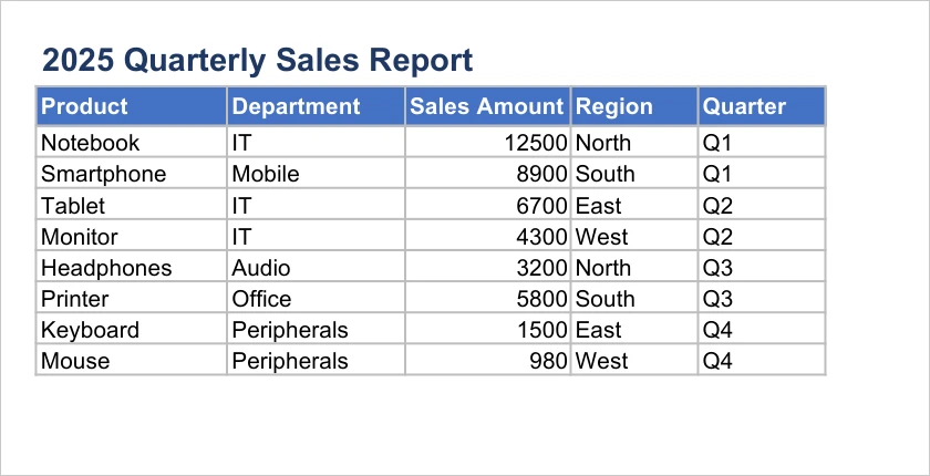
Because the watermark is carried by the header, removing it means clearing the reference in that header. Once the header text is empty, the image is no longer displayed and the body of the worksheet stays as it is.
Removing a watermark from an Excel worksheet:
| Syntax | Result |
|---|---|
workbook.LoadFromFile(...) |
Loads the watermarked workbook |
workbook.Worksheets.get(0) |
Gets the first worksheet to process |
sheet.PageSetup.LeftHeader = "" |
Clears the left header text and the image placeholder |
workbook.SaveToFile(...) |
Saves the workbook without the watermark to the VFS |
The steps are:
- Load the watermarked Excel file into the VFS.
- Create a
Workbookobject, load the document withLoadFromFile(), and get the first worksheet withWorkbook.Worksheets.get(0). - Set
PageSetup.LeftHeaderto an empty string to remove the watermark image placeholder from the header. - Use the
Workbook.SaveToFile()method to save the document, then release resources withWorkbook.Dispose().
Here is a complete code example showing how to remove a watermark from a worksheet in React:
function App() {
  const removeWatermark = async () => {
    // Get the Spire.XLS WASM module
    const xlsModule = window.wasmModule?.spirexls;

    // Check whether the module is ready
    if (!xlsModule) {
      alert('Spire.Xls is not ready yet');
      return;
    }

    // Load the watermarked Excel file into the VFS
    const inputFileName = 'AddWatermark.xlsx';
    await window.spire.FetchFileToVFS(inputFileName, '', `${process.env.PUBLIC_URL}data/`);

    // Load the workbook
    const workbook = new xlsModule.Workbook();
    workbook.LoadFromFile({ fileName: inputFileName });

    // Get the first worksheet
    const sheet = workbook.Worksheets.get(0);

    // Clear the left header text to remove the watermark
    sheet.PageSetup.LeftHeader = "";

    // Save the document
    const outputFileName = 'RemoveWatermark_output.xlsx';
    workbook.SaveToFile({ fileName: outputFileName, version: xlsModule.ExcelVersion.Version2010 });

    // Release resources
    workbook.Dispose();

    // Read the converted file from the VFS and trigger a download
    const fileArray = window.dotnetRuntime.Module.FS.readFile(outputFileName);
    const blob = new Blob([fileArray], { type: 'application/vnd.openxmlformats-officedocument.spreadsheetml.sheet' });
    const url = URL.createObjectURL(blob);
    const a = document.createElement('a');
    a.href = url;
    a.download = outputFileName;
    a.click();
    URL.revokeObjectURL(url);
  };

  return (
    <div style={{ textAlign: 'center', height: '300px' }}>
      <h1>Remove Watermark from Excel</h1>
      <button onClick={removeWatermark}>
        Start
      </button>
    </div>
  );
}

export default App;
The worksheet after removing the watermark:
FAQ
The watermark is not visible in Normal view
Cause: A watermark implemented through a header image is only displayed in Page Layout view and print preview, and is not visible in Excel's Normal view.
Solution: Switch the worksheet view to Page Layout mode to preview the watermark, for example by setting sheet.ViewMode = xlsModule.ViewMode.Layout in the code.
The watermark position is different from expected
Cause: A header image watermark is displayed in the header area, and its horizontal position can be controlled by the left, center, and right header positions. If the position does not match expectations, it is usually because the header position set is inconsistent with the requirement.
Solution: Choose LeftHeaderImage, CenterHeaderImage, or RightHeaderImage to set the watermark image according to your needs, and set the corresponding image placeholder &G with the LeftHeader, CenterHeader, or RightHeader property.
Residual content remains in the file after removing the watermark
Cause: The watermark is implemented through a header image. If only part of the header area is cleared, other areas (such as the left or right header) may still contain the watermark image.
Solution: Make sure to clear the text of all header areas where the watermark was set, including LeftHeader, CenterHeader, and RightHeader.
Obtain a Free License
Spire.XLS for JavaScript offers a 30-day full-featured free trial license with no functional limitations. Apply here to evaluate before purchasing.
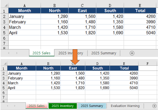
When a workbook holds several worksheets, default names and look-alike tabs make it hard to tell one sheet from another. Renaming “Sheet1” to “Quarterly Sales” tells a colleague at a glance what the sheet contains; marking the sales, inventory and summary sheets with red, green and light blue tabs removes the need to open each one while switching. Both the name and the tab color live inside the workbook itself, so they survive distribution and archiving without any external notes. Spire.XLS for JavaScript performs these operations in the browser through WebAssembly, managing input and output files with a virtual file system (VFS) and requiring no backend service.
This article covers two core features:
For installation and project setup, see Integrating Spire.XLS for JavaScript in a React Project. The examples below assume Spire.XLS is installed and the WebAssembly module has been initialized.
Rename Excel Worksheets
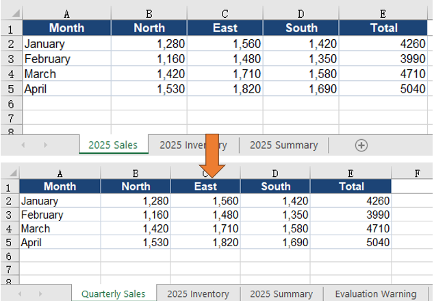
A worksheet name is the first identifier a reader sees after opening the file. With default names such as “Sheet1” and “Sheet2”, even a well-filled workbook has to be opened sheet by sheet before the right table turns up; with a business name such as “Quarterly Sales”, the tab strip itself becomes a table of contents, and the label is preserved when the file is printed or exported. The sample workbook contains sales, inventory and summary data in that order. This section renames the first worksheet.
How to rename a worksheet and what it produces:
| Call | Result |
|---|---|
workbook.Worksheets.get(0) |
Takes the first worksheet by index |
sheet.Name |
Reads back the current worksheet name |
sheet.Name = 'Quarterly Sales' |
Assigns the new worksheet name |
workbook.SaveToFile |
Saves the renamed workbook to the VFS |
The steps are:
- Load the font file and the test data file into the VFS with
window.spire.FetchFileToVFS. - Create a workbook with
new Workbook()and load the input file withworkbook.LoadFromFile. - Take the first worksheet with
workbook.Worksheets.get(0). - Assign the new name to
sheet.Name. - Save the workbook with
workbook.SaveToFile, then release the workbook object withworkbook.Dispose.
The complete example below renames an Excel worksheet in React:
function App() {
  const renameWorksheet = async () => {
    // Get the Spire.XLS WASM module
    const xlsModule = window.wasmModule?.spirexls;

    // Check that the module is ready
    if (!xlsModule) {
      alert('Spire.Xls is not ready yet');
      return;
    }

    // Load the font and the test data file into the VFS
    await window.spire.FetchFileToVFS('ARIAL.TTF', '/Library/Fonts/', `${process.env.PUBLIC_URL}/font/`);
    const inputFileName = 'WorksheetNames.xlsx';
    await window.spire.FetchFileToVFS(inputFileName, '', `${process.env.PUBLIC_URL}data/`);

    // Load the workbook and take the first worksheet
    const workbook = new xlsModule.Workbook();
    workbook.LoadFromFile({ fileName: inputFileName });
    const sheet = workbook.Worksheets.get(0);

    // Assign the new worksheet name
    sheet.Name = 'Quarterly Sales';

    // Save the workbook
    const outputFileName = 'RenameWorksheet.xlsx';
    workbook.SaveToFile({ fileName: outputFileName });

    // Dispose of the workbook to release its resources
    workbook.Dispose();

    // Read the result back out of the VFS and trigger the download
    const fileArray = window.dotnetRuntime.Module.FS.readFile(outputFileName);
    const blob = new Blob([fileArray], { type: 'application/vnd.openxmlformats-officedocument.spreadsheetml.sheet' });
    const url = URL.createObjectURL(blob);
    const a = document.createElement('a');
    a.href = url;
    a.download = outputFileName;
    a.click();
    URL.revokeObjectURL(url);
  };

  return (
    <div style={{ textAlign: 'center', height: '300px' }}>
      <h1>Rename Excel Worksheets</h1>
      <button id="rename-worksheet" onClick={renameWorksheet}>Rename Worksheet</button>
    </div>
  );
}

export default App;
The workbook after renaming the first worksheet:
Set Excel Worksheet Tab Colors
Even with descriptive names, the tab strip remains a row of similarly sized text, which has to be scanned sheet by sheet. Tab colors add a second identifier: red for sales, green for inventory and light blue for summary. Color is perceived before the text is read, so a reader can locate a group directly, and both the color and the name stay in the workbook when the file is shared. The three worksheets in the sample correspond to the three groups, so this section assigns each one a different tab color.
How to set worksheet tab colors and what it produces:
| Call | Result |
|---|---|
workbook.Worksheets.get(0) |
Takes the worksheet whose tab will be colored |
sheet.TabColor = xlsModule.Color.get_Red() |
Turns the worksheet tab red |
sheet.TabColor = xlsModule.Color.get_Green() |
Turns the worksheet tab green |
sheet.TabColor = xlsModule.Color.get_LightBlue() |
Turns the worksheet tab light blue |
xlsModule.Color.FromArgb(255, 255, 193, 7) |
Builds a custom RGB color for TabColor |
The steps are:
- Load the font file and the test data file into the VFS with
window.spire.FetchFileToVFS. - Create a workbook with
new Workbook()and load the input file withworkbook.LoadFromFile. - Take the three worksheets in order with
workbook.Worksheets.get(0),get(1)andget(2). - Assign
xlsModule.Color.get_Red(),get_Green()andget_LightBlue()to each worksheet'sTabColor. - Save the workbook with
workbook.SaveToFile, then release the workbook object withworkbook.Dispose.
The complete example below sets worksheet tab colors in React:
function App() {
  const setTabColor = async () => {
    // Get the Spire.XLS WASM module
    const xlsModule = window.wasmModule?.spirexls;

    // Check that the module is ready
    if (!xlsModule) {
      alert('Spire.Xls is not ready yet');
      return;
    }

    // Load the font and the test data file into the VFS
    await window.spire.FetchFileToVFS('ARIAL.TTF', '/Library/Fonts/', `${process.env.PUBLIC_URL}/font/`);
    const inputFileName = 'WorksheetNames.xlsx';
    await window.spire.FetchFileToVFS(inputFileName, '', `${process.env.PUBLIC_URL}data/`);

    // Load the workbook
    const workbook = new xlsModule.Workbook();
    workbook.LoadFromFile({ fileName: inputFileName });

    // Set the tab colours to red, green and light blue in worksheet order
    workbook.Worksheets.get(0).TabColor = xlsModule.Color.get_Red();
    workbook.Worksheets.get(1).TabColor = xlsModule.Color.get_Green();
    workbook.Worksheets.get(2).TabColor = xlsModule.Color.get_LightBlue();

    // Save the workbook
    const outputFileName = 'SetTabColor.xlsx';
    workbook.SaveToFile({ fileName: outputFileName });

    // Dispose of the workbook to release its resources
    workbook.Dispose();

    // Read the result back out of the VFS and trigger the download
    const fileArray = window.dotnetRuntime.Module.FS.readFile(outputFileName);
    const blob = new Blob([fileArray], { type: 'application/vnd.openxmlformats-officedocument.spreadsheetml.sheet' });
    const url = URL.createObjectURL(blob);
    const a = document.createElement('a');
    a.href = url;
    a.download = outputFileName;
    a.click();
    URL.revokeObjectURL(url);
  };

  return (
    <div style={{ textAlign: 'center', height: '300px' }}>
      <h1>Set Excel Worksheet Tab Colors</h1>
      <button id="set-tab-color" onClick={setTabColor}>Set Tab Colors</button>
    </div>
  );
}

export default App;
The workbook after setting tab colors for the three worksheets:
Set a Custom Tab Color
When the built-in colors do not fit a report's palette, Color.FromArgb builds a custom color. Its four arguments are the alpha, red, green and blue channels, each from 0 to 255:
// Set the first worksheet tab to amber
workbook.Worksheets.get(0).TabColor = xlsModule.Color.FromArgb(255, 255, 193, 7);
FAQ
Worksheet rename reports a duplicate name
Cause: Worksheet names in a workbook must be unique, and the comparison ignores case. Assigning a name already used by another worksheet, such as “Sales” and “sales”, triggers the limit.
Solution: Before renaming, iterate over workbook.Worksheets, read each Name, and confirm the target name is free before assigning it to sheet.Name.
A sheet name containing a slash throws an error
Cause: Excel does not allow worksheet names to contain :, \, /, ?, *, [ or ]; Spire.XLS throws when such a name is assigned.
Solution: Replace the illegal characters with a hyphen or underscore before assigning the value to sheet.Name.
What happens when a worksheet name exceeds 31 characters
Cause: Excel limits worksheet names to 31 characters. Spire.XLS does not report an error; it truncates the name to 31 characters before writing it.
Solution: Check name.length before assigning and shorten the name when it is longer than 31 characters. The truncation happens during assignment, so comparing the saved name with the intended one will reveal the difference.
Getting a worksheet by name throws Arg_NullReferenceException
Cause: workbook.Worksheets.get('name') returns a worksheet only when the name matches exactly. A missing name, a trailing space, or a worksheet that has already been renamed all throw this exception.
Solution: Iterate over workbook.Worksheets and print each Name to confirm the current name before calling get. When the name comes from external input, trim leading and trailing spaces first.
Get a Free License
Spire.XLS for JavaScript offers a 30-day full-featured free trial license with no functional limitations. Apply here to evaluate before purchasing.
UOS is the spreadsheet format of the UOF specification, saved with the .uos extension, and office suites that implement the specification can open it directly. When an Excel report is handed to such an environment and .xlsx is not supported, the workbook has to be converted to UOS first; a UOS file received in return has to be converted back to Excel before it can be edited in the usual tools. Conversion only changes the saved format: formulas, merged areas, number formats and text formatting travel with the file. Spire.XLS for JavaScript performs the conversion in the browser through WebAssembly, and the input and output files are managed by a virtual file system (VFS), with no backend service required.
This article covers two feature points:
For installation and project setup, see Integrating Spire.XLS for JavaScript in a React Project. The examples below assume Spire.XLS is installed and the WebAssembly module has been initialized.
Convert Excel to UOS
Saving an Excel workbook as UOS lets an office suite that only recognizes the UOF format open the report directly. Only the saved format changes; worksheet names, merged areas and number formats stay as they are. Formula cells need one extra step: they have to be calculated before saving so that both the formula and its result are written.
How to convert Excel to UOS and what it produces:
| Call | Result |
|---|---|
window.spire.FetchFileToVFS |
Loads the font file and the Excel file into the virtual file system |
workbook.LoadFromFile({ fileName }) |
Loads the Excel workbook |
workbook.CalculateAllValue() |
Calculates every formula in the workbook |
xlsModule.FileFormat.UOS |
Sets the target format to UOS |
workbook.SaveToFile({ fileName, fileFormat }) |
Writes the workbook to the virtual file system in UOS format |
The steps are:
- Load the font file and the Excel test file into the VFS with
window.spire.FetchFileToVFS. - Create a workbook with
new Workbook()and load the test file withworkbook.LoadFromFile. - Calculate the formulas with
workbook.CalculateAllValue(). - Call
workbook.SaveToFilewithfileFormatset toxlsModule.FileFormat.UOS, writingExcelToUos.uos. - Release the workbook with
workbook.Dispose, then read the result out of the VFS and trigger the download.
The following is a complete code example that shows how to convert an Excel workbook to UOS in React:
function App() {
  const excelToUos = async () => {
    // Get the Spire.XLS WASM module
    const xlsModule = window.wasmModule?.spirexls;

    // Check that the module is ready
    if (!xlsModule) {
      alert('Spire.Xls is not ready yet');
      return;
    }

    // Load the font and the test data file into the VFS
    await window.spire.FetchFileToVFS('ARIAL.TTF', '/Library/Fonts/', `${process.env.PUBLIC_URL}/font/`);
    const inputFileName = 'SalesReport.xlsx';
    await window.spire.FetchFileToVFS(inputFileName, '', `${process.env.PUBLIC_URL}data/`);

    // Load the workbook
    const workbook = new xlsModule.Workbook();
    workbook.LoadFromFile({ fileName: inputFileName });

    // Calculate the formulas so the formula cells carry their results
    workbook.CalculateAllValue();

    // Save as UOS, with the format given by fileFormat
    const outputFileName = 'ExcelToUos.uos';
    workbook.SaveToFile({ fileName: outputFileName, fileFormat: xlsModule.FileFormat.UOS });

    // Dispose of the workbook to release its resources
    workbook.Dispose();

    // Read the result back out of the VFS and trigger the download
    const fileArray = window.dotnetRuntime.Module.FS.readFile(outputFileName);
    const blob = new Blob([fileArray], { type: 'application/octet-stream' });
    const url = URL.createObjectURL(blob);
    const a = document.createElement('a');
    a.href = url;
    a.download = outputFileName;
    a.click();
    URL.revokeObjectURL(url);
  };

  return (
    <div style={{ textAlign: 'center', height: '300px' }}>
      <h1>Convert Between Excel and UOS in React</h1>
      <button id="excel-to-uos" onClick={excelToUos}>Convert Excel to UOS</button>
    </div>
  );
}

export default App;
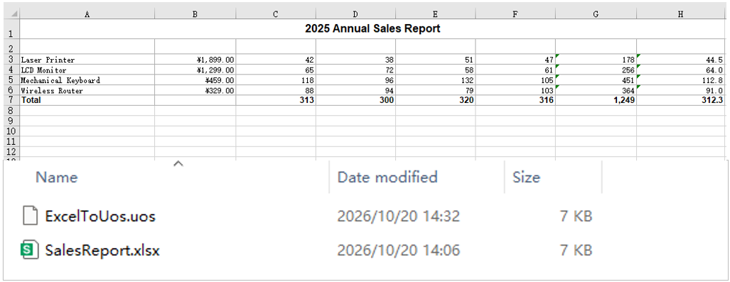
The UOS file produced from the Excel workbook:
Convert UOS to Excel
Converting a received UOS file back to Excel is the reverse of the same process. UOS and Excel store the same workbook content; loading restores worksheet names, cell data and styles, and formulas come back together with their cached results, so nothing has to be recalculated before saving. The converted file can then be opened in Excel or an online spreadsheet tool for further editing, summarizing or printing.
How to convert a UOS file to Excel and what it produces:
| Call | Result |
|---|---|
window.spire.FetchFileToVFS |
Loads the font file and the UOS file into the virtual file system |
workbook.LoadFromFile({ fileName }) |
Reads the UOS file and recognizes it as a workbook |
xlsModule.FileFormat.Version2010 |
Sets the target format to Excel 2010 or later |
workbook.SaveToFile({ fileName, fileFormat }) |
Writes the workbook to the virtual file system in Excel format |
window.dotnetRuntime.Module.FS.readFile |
Reads the result out of the VFS and triggers the download |
The steps are:
- Load the font file and the UOS test file into the VFS with
window.spire.FetchFileToVFS. - Create a workbook with
new Workbook()and load the UOS file withworkbook.LoadFromFile. - Call
workbook.SaveToFilewithfileFormatset toxlsModule.FileFormat.Version2010, writingUosToExcel.xlsx. - Release the workbook with
workbook.Dispose, then read the result out of the VFS and trigger the download.
The following is a complete code example that shows how to convert a UOS file back to Excel in React:
function App() {
  const uosToExcel = async () => {
    // Get the Spire.XLS WASM module
    const xlsModule = window.wasmModule?.spirexls;

    // Check that the module is ready
    if (!xlsModule) {
      alert('Spire.Xls is not ready yet');
      return;
    }

    // Load the font and the test data file into the VFS
    await window.spire.FetchFileToVFS('ARIAL.TTF', '/Library/Fonts/', `${process.env.PUBLIC_URL}/font/`);
    const inputFileName = 'SalesReport.uos';
    await window.spire.FetchFileToVFS(inputFileName, '', `${process.env.PUBLIC_URL}data/`);

    // Load the UOS file
    const workbook = new xlsModule.Workbook();
    workbook.LoadFromFile({ fileName: inputFileName });

    // Save as Excel, with the version given by fileFormat
    const outputFileName = 'UosToExcel.xlsx';
    workbook.SaveToFile({ fileName: outputFileName, fileFormat: xlsModule.FileFormat.Version2010 });

    // Dispose of the workbook to release its resources
    workbook.Dispose();

    // Read the result back out of the VFS and trigger the download
    const fileArray = window.dotnetRuntime.Module.FS.readFile(outputFileName);
    const blob = new Blob([fileArray], { type: 'application/vnd.openxmlformats-officedocument.spreadsheetml.sheet' });
    const url = URL.createObjectURL(blob);
    const a = document.createElement('a');
    a.href = url;
    a.download = outputFileName;
    a.click();
    URL.revokeObjectURL(url);
  };

  return (
    <div style={{ textAlign: 'center', height: '300px' }}>
      <h1>Convert Between Excel and UOS in React</h1>
      <button id="uos-to-excel" onClick={uosToExcel}>Convert UOS to Excel</button>
    </div>
  );
}

export default App;
The workbook produced from the UOS file:
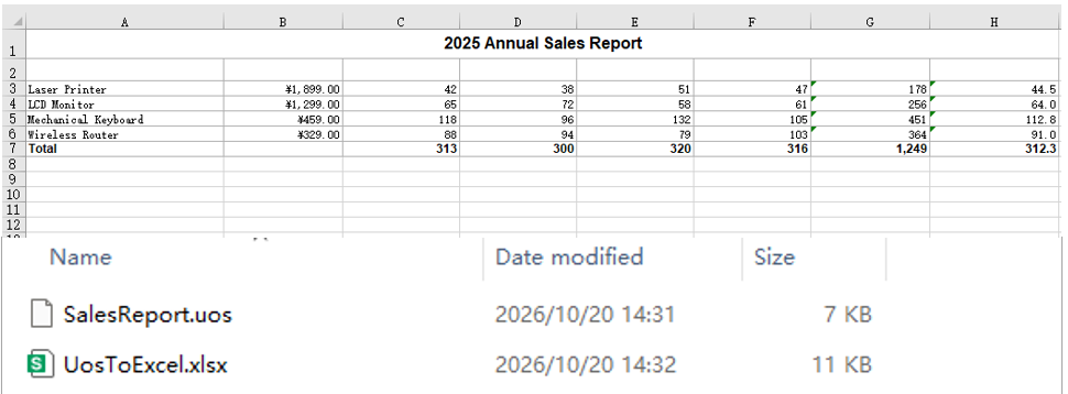
FAQ
Why are the formula cells empty in the UOS file after conversion
Cause: During export, the formula and the value of each cell are taken from the workbook's current calculation results. If CalculateAllValue has not been called after loading, the formula cells are still uncalculated and are written as empty cells, so neither the formula nor the value survives.
Solution: Call workbook.CalculateAllValue() after workbook.LoadFromFile and before workbook.SaveToFile, then save with FileFormat.UOS; the formula cells will carry both the formula and the calculated result.
Can I save as UOS by using only the .uos extension without fileFormat
Cause: fileFormat is an optional parameter of SaveToFile. When it is omitted, the save format is inferred from the extension of the output file name, and a recognizable extension selects that format.
Solution: Yes. Name the output file ExcelToUos.uos and call workbook.SaveToFile({ fileName: outputFileName }); the file is still written as UOS. Setting fileFormat explicitly is safer, because a missing or misspelled extension will not silently produce another format.
Get a Free License
Spire.XLS for JavaScript offers a 30-day full-featured free trial license with no functional limitations. Apply here to evaluate before purchasing.
Add a Data Table to an Excel Chart with JavaScript in React
2026-10-19 09:00:23 Written by liu taliaA chart makes a trend visible at a glance, yet it does not give the exact numbers: the height of a column has to be read against the value axis, and the estimate drifts as more series crowd in. A data table lists the category names, series names and values directly below the chart, so readers do not have to go back to the source cells or add a data label to every point. As part of the chart, the table scales and moves with it and stays in place when the chart is exported as an image or printed. Spire.XLS for JavaScript performs these operations in the browser through WebAssembly; the input and output files are managed by a virtual file system (VFS), with no backend service required.
This article covers two feature points:
For installation and project setup, see Integrating Spire.XLS for JavaScript in a React Project. The examples below assume Spire.XLS is installed and the WebAssembly module has been initialized.
Add a data table to the chart
Adding a data table to a chart solves the problem of numbers living apart from the picture. A default column chart only draws the columns; the values stay in the source worksheet and the reader has to move between the two. With several series, a data table sits directly under the category axis, one row per series, its columns aligned with the categories and its rows matching the colours in the legend, so the trend and the figures appear in one place. The sample workbook already holds a quarterly sales table and a column chart; what it lacks is the table below the chart.
Turning the data table on:
| Syntax | Result |
|---|---|
workbook.Worksheets.get(0) |
Takes the first worksheet of the workbook |
sheet.Charts.get(0) |
Takes the first chart on the worksheet |
chart.HasDataTable = true |
Shows a data table below the chart with the categories, series names and values |
workbook.SaveToFile |
Saves the workbook with its data table into the VFS |
The steps are:
- Load the font file and the test data file into the VFS with
window.spire.FetchFileToVFS. - Create a workbook with
new Workbook(), load the input file withworkbook.LoadFromFile, and take the first worksheet withworkbook.Worksheets.get(0). - Take the first chart on the worksheet with
sheet.Charts.get(0). - Set
chart.HasDataTabletotrue, which adds the data table below the chart. - Save the workbook with
workbook.SaveToFileand dispose of it withworkbook.Disposeto free resources.
The full code example below shows how to add a data table to an Excel chart in React:
function App() {
  const addDataTable = async () => {
    // Get the Spire.XLS WASM module
    const xlsModule = window.wasmModule?.spirexls;

    // Check that the module is ready
    if (!xlsModule) {
      alert('Spire.Xls is not ready yet');
      return;
    }

    // Load the font and the test data file into the VFS
    await window.spire.FetchFileToVFS('ARIAL.TTF', '/Library/Fonts/', `${process.env.PUBLIC_URL}/font/`);
    const inputFileName = 'ChartSales.xlsx';
    await window.spire.FetchFileToVFS(inputFileName, '', `${process.env.PUBLIC_URL}data/`);

    // Load the workbook and take the first worksheet and its chart
    const workbook = new xlsModule.Workbook();
    workbook.LoadFromFile({ fileName: inputFileName });
    const sheet = workbook.Worksheets.get(0);
    const chart = sheet.Charts.get(0);

    // Turn on the chart's data table, which lists the categories and series values below the plot
    chart.HasDataTable = true;

    // Save the workbook
    const outputFileName = 'AddDataTable.xlsx';
    workbook.SaveToFile({ fileName: outputFileName });

    // Dispose of the workbook to release its resources
    workbook.Dispose();

    // Read the result back out of the VFS and trigger the download
    const fileArray = window.dotnetRuntime.Module.FS.readFile(outputFileName);
    const blob = new Blob([fileArray], { type: 'application/vnd.openxmlformats-officedocument.spreadsheetml.sheet' });
    const url = URL.createObjectURL(blob);
    const a = document.createElement('a');
    a.href = url;
    a.download = outputFileName;
    a.click();
    URL.revokeObjectURL(url);
  };

  return (
    <div style={{ textAlign: 'center', height: '300px' }}>
      <h1>Add a Data Table to an Excel Chart</h1>
      <button id="add-data-table" onClick={addDataTable}>Add a Data Table to the Chart</button>
    </div>
  );
}

export default App;
The sales report after turning on the chart data table:
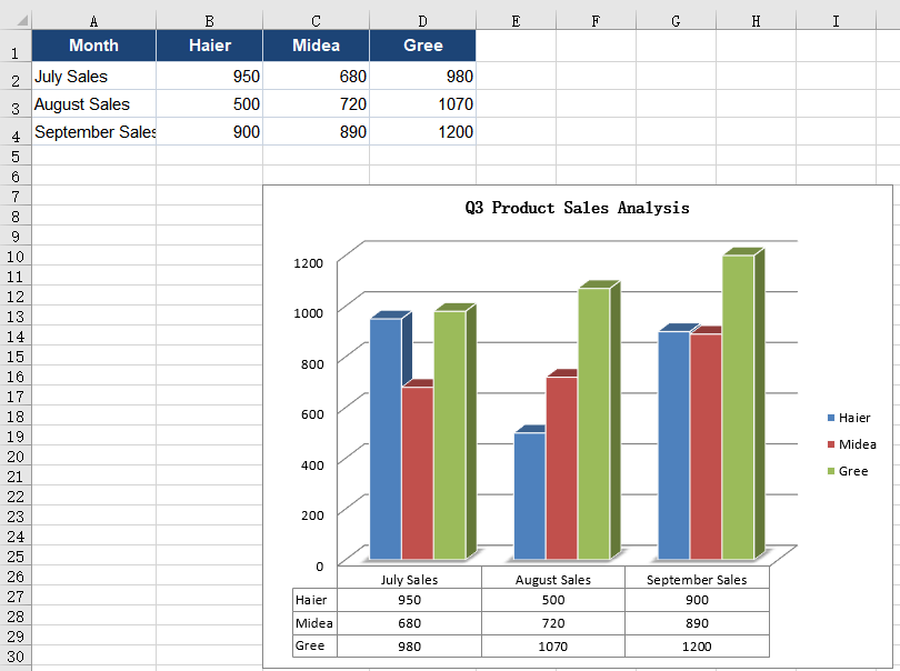
Adjust the data table borders, legend keys and text formatting
Adjusting the data table borders, legend keys and text formatting keeps the table readable when there are many series and lets it blend into the layout of a report. A newly opened data table carries an outer frame and both horizontal and vertical separators; with three rows of values stacked together it looks like a dense grid. Dropping the outer frame and the vertical lines leaves only the horizontal ones, so the eye follows a row straight to its numbers without being cut off by vertical rules. Turning on the legend keys then puts a colour swatch of the matching series in front of every series name, so readers no longer have to compare each row with the legend. By default the text draws on the chart's own settings -- ten points, black, not bold -- which does not stand out against dark columns and gridlines; dropping the size to nine points fits more numbers on a line, while bolding the text and switching it to a deeper blue ties it to the title and the header row. These settings apply to the data table alone; the chart title, axis labels and legend keep their own fonts.
Borders, legend keys and text formatting:
| Syntax | Result |
|---|---|
chart.DataTable |
Takes the data table object of the chart |
table.HasBorders = false |
Removes the outer frame of the data table |
table.HasVertBorder = false |
Removes the vertical separators between columns |
table.HasHorzBorder = true |
Keeps the horizontal separators between rows |
table.ShowSeriesKeys = true |
Shows a legend key in front of every series name |
table.FontName = 'Arial' |
Sets the data table text to Arial |
table.Size = 9 |
Sets the data table text to 9 points |
table.IsBold = true |
Bolds the data table text |
table.Color = xlsModule.Color.FromArgb(255, 28, 68, 118) |
Sets the data table text to a deep blue |
The steps are:
- Load the font and the test data file into the VFS with
window.spire.FetchFileToVFS, then load the workbook withworkbook.LoadFromFile. - Take the first worksheet with
workbook.Worksheets.get(0)and the first chart withsheet.Charts.get(0). - Set
chart.HasDataTabletotrueto open the data table, then take the object withchart.DataTable. - Set
table.HasBordersandtable.HasVertBordertofalseandtable.HasHorzBordertotrue, so only the horizontal lines remain. - Set
table.ShowSeriesKeystotrueto show the legend key before each series name. - Set
table.FontName,table.Sizeandtable.IsBoldto choose the typeface, the size and the bold weight. - Build a deep blue with
xlsModule.Color.FromArgband assign it totable.Color. - Save the workbook with
workbook.SaveToFileand dispose of it withworkbook.Disposeto free resources.
The full code example below shows how to adjust the data table borders, legend keys and text formatting in React:
function App() {
  const customizeDataTable = async () => {
    // Get the Spire.XLS WASM module
    const xlsModule = window.wasmModule?.spirexls;

    // Check that the module is ready
    if (!xlsModule) {
      alert('Spire.Xls is not ready yet');
      return;
    }

    // Load the font and the test data file into the VFS
    await window.spire.FetchFileToVFS('ARIAL.TTF', '/Library/Fonts/', `${process.env.PUBLIC_URL}/font/`);
    const inputFileName = 'ChartSales.xlsx';
    await window.spire.FetchFileToVFS(inputFileName, '', `${process.env.PUBLIC_URL}data/`);

    // Load the workbook and take the first worksheet and its chart
    const workbook = new xlsModule.Workbook();
    workbook.LoadFromFile({ fileName: inputFileName });
    const sheet = workbook.Worksheets.get(0);
    const chart = sheet.Charts.get(0);

    // Turn on the data table and take its object
    chart.HasDataTable = true;
    const table = chart.DataTable;

    // Drop the outer frame and the vertical lines, keeping only the horizontal ones
    table.HasBorders = false;
    table.HasVertBorder = false;
    table.HasHorzBorder = true;

    // Show the legend key in front of each series name
    table.ShowSeriesKeys = true;

    // Set the data table font, size, bold weight and text colour
    table.FontName = 'Arial';
    table.Size = 9;
    table.IsBold = true;
    table.Color = xlsModule.Color.FromArgb(255, 28, 68, 118);

    // Save the workbook
    const outputFileName = 'DataTableFormatting.xlsx';
    workbook.SaveToFile({ fileName: outputFileName });

    // Dispose of the workbook to release its resources
    workbook.Dispose();

    // Read the result back out of the VFS and trigger the download
    const fileArray = window.dotnetRuntime.Module.FS.readFile(outputFileName);
    const blob = new Blob([fileArray], { type: 'application/vnd.openxmlformats-officedocument.spreadsheetml.sheet' });
    const url = URL.createObjectURL(blob);
    const a = document.createElement('a');
    a.href = url;
    a.download = outputFileName;
    a.click();
    URL.revokeObjectURL(url);
  };

  return (
    <div style={{ textAlign: 'center', height: '300px' }}>
      <h1>Add a Data Table to an Excel Chart</h1>
      <button id="data-table-formatting" onClick={customizeDataTable}>Adjust the Borders, Legend Keys and Text</button>
    </div>
  );
}

export default App;
The data table after adjusting the borders, legend keys and text formatting:
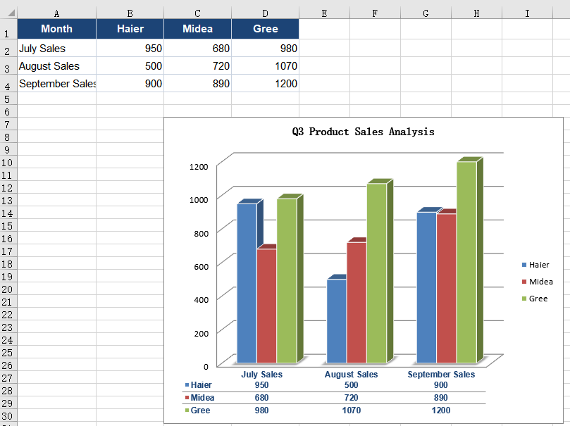
FAQ
What is the difference between a data table and data labels?
Cause: Data labels sit next to each data point and show only that point's value. A data table sits below the chart, one row per series, and gives the category names and all the values together.
Solution: Use data labels when each point needs a callout without a table taking up space; use a data table when readers should take in a whole set of values at once. Both can be present on the same chart and turned on or off as needed.
How do I remove the data table from a chart?
Cause: The data table is controlled by a single switch on the chart; once it is on, it does not disappear with a change of source data or chart type.
Solution: Set chart.HasDataTable to false and save the workbook; the data table below the chart is removed.
How can the data table use a different font from the rest of the chart?
Cause: The data table carries its own text formatting. Until it is set, it follows the rest of the chart's text; once set, only the data table changes.
Solution: Set FontName, Size, IsBold and Color on chart.DataTable. These properties act on the data table only and leave the chart title, axis labels and legend untouched.
What is the legend key in a data table?
Cause: A legend key is the small colour swatch shown in front of a series name, matching the series' marker in the legend. It is off by default, so the data table shows plain text.
Solution: Set table.ShowSeriesKeys to true; a swatch then appears in front of every series name, so a reader can match a row of the data table with the legend directly.
Get a Free License
Spire.XLS for JavaScript offers a 30-day full-featured free trial license with no functional limitations. Apply here to evaluate before purchasing.
Text boxes in a worksheet carry notices, reminders or a single conclusion, yet their default look is plain: small black text on white, framed by a thin border that blends into the grid. Enlarging and bolding the font and laying down a light fill make the text rise above the table; inner margins and text wrapping keep long sentences off the border and inside the box; removing the border lets a text box read as a quiet annotation. These changes can be applied in code in one pass instead of one box at a time. Spire.XLS for JavaScript runs in the browser on WebAssembly and handles the input and output files through a virtual file system (VFS), with no backend service required.
This article covers two core feature points:
- Adjust the Font, Background and Border of Text Boxes
- Set the Inner Margins and Text Wrapping of Text Boxes
For installation and project setup, see Integrating Spire.XLS for JavaScript in a React Project. The examples below assume Spire.XLS is installed and the WebAssembly module has been initialised.
Adjust the Font, Background and Border of Text Boxes
The default 11-point black text on a white background lacks contrast against the sheet. A larger size, a bold weight, another color and a pale fill lift a notice above the grid; clearing a border that competes with the cell lines makes the text read as if written straight on the page, which suits footnotes and corner notes. The same two kinds of change can be applied to one text box or split across different boxes, and this feature point adjusts the font, background and border of text boxes.
| Syntax | Result |
|---|---|
workbook.CreateFont() |
Creates a font object for the text of a text box |
font.FontName, font.Size, font.IsBold, font.Color |
Set the font name, size, bold weight and text color |
xlsModule.RichTextShape.Convert(textBox.RichText) |
Returns the rich text object of the text box |
richText.SetFont(0, textBox.Text.length - 1, font) |
Applies the font to the whole text of the text box |
textBox.Fill.FillType = xlsModule.ShapeFillType.SolidColor |
Switches the text box background to a solid fill |
textBox.Fill.ForeColor |
Sets the color of the solid fill |
textBox.Line.Weight = 0 |
Sets the border weight to zero, so no outline is drawn |
The steps are:
- Take the first text box with
sheet.TextBoxes.get(0). - Create a font object with
workbook.CreateFont()and set its name, size, bold weight and color throughFontName,Size,IsBoldandColor. - Get the rich text object with
xlsModule.RichTextShape.Convert(textBox.RichText), then callSetFont(0, textBox.Text.length - 1, font)to apply the font to the whole text. - Set
textBox.Fill.FillTypetoxlsModule.ShapeFillType.SolidColor, then name the fill color withtextBox.Fill.ForeColor. - Take the fourth text box with
sheet.TextBoxes.get(3)and settextBox.Line.Weightto0to remove its border. - Save the workbook with
workbook.SaveToFile.
The code below is the complete example of adjusting the font, background and border of a text box:
function App() {
  const adjustTextAppearance = async () => {
    // get the Spire.XLS WASM module
    const xlsModule = window.wasmModule?.spirexls;

    // check that the module is ready
    if (!xlsModule) {
      alert('Spire.Xls is not ready yet');
      return;
    }

    // load the font and the test data file into the VFS
    await window.spire.FetchFileToVFS('ARIAL.TTF', '/Library/Fonts/', `${process.env.PUBLIC_URL}/font/`);
    const inputFileName = 'TextBoxSample.xlsx';
    await window.spire.FetchFileToVFS(inputFileName, '', `${process.env.PUBLIC_URL}data/`);

    // load the workbook and take the first worksheet
    const workbook = new xlsModule.Workbook();
    workbook.LoadFromFile({ fileName: inputFileName });
    const sheet = workbook.Worksheets.get(0);

    // take the first text box and create a font with its name, size, bold weight and color
    const textBox = sheet.TextBoxes.get(0);
    const font = workbook.CreateFont();
    font.FontName = 'Arial';
    font.Size = 14;
    font.IsBold = true;
    font.Color = xlsModule.Color.FromArgb(255, 28, 68, 118);

    // apply the font to all the text in the text box
    const richText = xlsModule.RichTextShape.Convert(textBox.RichText);
    richText.SetFont(0, textBox.Text.length - 1, font);

    // fill the text box background with a solid color
    textBox.Fill.FillType = xlsModule.ShapeFillType.SolidColor;
    textBox.Fill.ForeColor = xlsModule.Color.FromArgb(255, 232, 240, 250);

    // take the fourth text box and set the border weight to 0, which removes the border
    const borderBox = sheet.TextBoxes.get(3);
    borderBox.Line.Weight = 0;

    // save the workbook
    const outputFileName = 'TextAppearance.xlsx';
    workbook.SaveToFile({ fileName: outputFileName });

    // dispose of the workbook to release its resources
    workbook.Dispose();

    // read the result back out of the VFS and trigger the download
    const fileArray = window.dotnetRuntime.Module.FS.readFile(outputFileName);
    const blob = new Blob([fileArray], { type: 'application/vnd.openxmlformats-officedocument.spreadsheetml.sheet' });
    const url = URL.createObjectURL(blob);
    const a = document.createElement('a');
    a.href = url;
    a.download = outputFileName;
    a.click();
    URL.revokeObjectURL(url);
  };

  return (
    <div style={{ textAlign: 'center', height: '300px' }}>
      <h1>Format Excel Text Boxes</h1>
      <button onClick={adjustTextAppearance}>Adjust the Font, Background and Border of a Text Box</button>
    </div>
  );
}

export default App;
The notice board after adjusting the font, background and border:
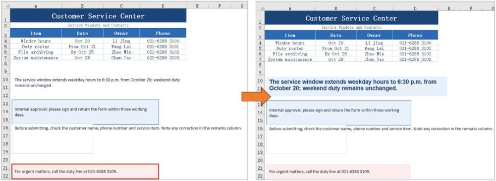
Set the Inner Margins and Text Wrapping of Text Boxes
Text pressed against the border is hard to read, especially on a dark fill. Inner margins hold the text away from each edge and can be set separately for the four sides. A long sentence in a narrow box stays on one line by default and runs past the border, while text wrapping folds it onto the next line. The sample leaves about 1 cm on the left and right and 0.4 cm at the top and bottom, and aligns the text to the top left so the shift caused by the margins is visible. This feature point sets the inner margins and text wrapping of text boxes.
| Syntax | Result |
|---|---|
textBox.InnerLeftMargin, InnerRightMargin, InnerTopMargin, InnerBottomMargin |
Set the distance between the text and the left, right, top and bottom border |
xlsModule.CommentHAlignType.Left |
Aligns the text to the left inside the box |
xlsModule.CommentVAlignType.Top |
Aligns the text to the top inside the box |
textBox.IsWrapText = true |
Folds the text onto the next line when it reaches the box width |
The steps are:
- Take the second text box with
sheet.TextBoxes.get(1). - Set
InnerLeftMargin,InnerRightMargin,InnerTopMarginandInnerBottomMarginin turn to leave room on all four sides. - Set
HAlignmenttoxlsModule.CommentHAlignType.LeftandVAlignmenttoxlsModule.CommentVAlignType.Top, so the text starts from the top-left corner. - Take the third text box with
sheet.TextBoxes.get(2)and setIsWrapTexttotrueto turn on text wrapping. - Save the workbook with
workbook.SaveToFile.
The code below is the complete example of setting the inner margins and text wrapping of a text box:
function App() {
  const setTextLayout = async () => {
    // get the Spire.XLS WASM module
    const xlsModule = window.wasmModule?.spirexls;

    // check that the module is ready
    if (!xlsModule) {
      alert('Spire.Xls is not ready yet');
      return;
    }

    // load the font and the test data file into the VFS
    await window.spire.FetchFileToVFS('ARIAL.TTF', '/Library/Fonts/', `${process.env.PUBLIC_URL}/font/`);
    const inputFileName = 'TextBoxSample.xlsx';
    await window.spire.FetchFileToVFS(inputFileName, '', `${process.env.PUBLIC_URL}data/`);

    // load the workbook and take the first worksheet
    const workbook = new xlsModule.Workbook();
    workbook.LoadFromFile({ fileName: inputFileName });
    const sheet = workbook.Worksheets.get(0);

    // take the second text box and set the space between the text and its four borders
    const textBox = sheet.TextBoxes.get(1);
    textBox.InnerLeftMargin = 1;
    textBox.InnerRightMargin = 1;
    textBox.InnerTopMargin = 0.4;
    textBox.InnerBottomMargin = 0.4;

    // align the text to the top left so the effect of the margins is visible
    textBox.HAlignment = xlsModule.CommentHAlignType.Left;
    textBox.VAlignment = xlsModule.CommentVAlignType.Top;

    // take the third text box and turn on wrapping, so text folds at the box width
    const wrapBox = sheet.TextBoxes.get(2);
    wrapBox.IsWrapText = true;

    // save the workbook
    const outputFileName = 'TextLayout.xlsx';
    workbook.SaveToFile({ fileName: outputFileName });

    // dispose of the workbook to release its resources
    workbook.Dispose();

    // read the result back out of the VFS and trigger the download
    const fileArray = window.dotnetRuntime.Module.FS.readFile(outputFileName);
    const blob = new Blob([fileArray], { type: 'application/vnd.openxmlformats-officedocument.spreadsheetml.sheet' });
    const url = URL.createObjectURL(blob);
    const a = document.createElement('a');
    a.href = url;
    a.download = outputFileName;
    a.click();
    URL.revokeObjectURL(url);
  };

  return (
    <div style={{ textAlign: 'center', height: '300px' }}>
      <h1>Format Excel Text Boxes</h1>
      <button onClick={setTextLayout}>Set the Inner Margins and Text Wrapping of a Text Box</button>
    </div>
  );
}

export default App;
The notice board after setting the inner margins and text wrapping:
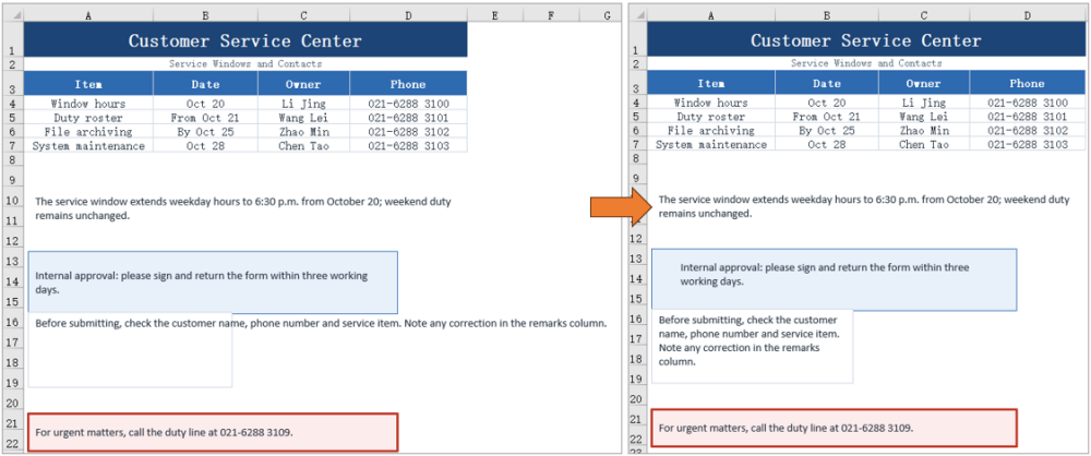
FAQ
How do I get a text box by name?
Cause: Getting text boxes by index means remembering their order in the collection, and inserting or removing a text box changes that order.
Solution: Use sheet.TextBoxes.get("TextBox 2") to get a text box by name.
How do I format only part of the text in a text box?
Cause: The text of a text box is stored as rich text, and SetFont applies to a character range; anything outside the range keeps its original format.
Solution: Get the rich text object with xlsModule.RichTextShape.Convert(textBox.RichText), then call richText.SetFont(startIndex, endIndex, font) with the range you want. For example, SetFont(0, 3, font) applies to the first four characters only.
Can the border of a text box have another color or a dashed style?
Cause: Besides its weight, the Line object also provides color and dash style settings.
Solution: Set the border color with textBox.Line.ForeColor, the weight with textBox.Line.Weight, and the dash style with textBox.Line.DashStyle, whose value is a member of xlsModule.ShapeDashLineStyleType, such as Dashed for a dashed line.
What if the text does not wrap as expected?
Cause: Text only wraps when IsWrapText is true, and when the text box is wide enough for the whole sentence no line break appears either.
Solution: Confirm that textBox.IsWrapText = true has been set, and check that the width of the text box is smaller than the length of the sentence. When several lines are needed, leave enough height in the text box as well.
Get a Free License
Spire.XLS for JavaScript offers a 30-day full-featured free trial license with no functional limitations. Apply here to evaluate before purchasing.
A cell whose formatting is already right often has to be reused elsewhere: the unit price column carries a money format, a light blue fill and thin borders, while the amount column on the same row is still plain. Copying a cell format hands the look the source cell has already settled on to the target cell -- number format, font, fill, border and alignment in one go -- and leaves the data in the target cell untouched. Spire.XLS for JavaScript performs these operations in the browser through WebAssembly; the input and output files are managed by a virtual file system (VFS), with no backend service required.
This article covers two feature points:
For installation and project setup, see Integrating Spire.XLS for JavaScript in a React Project. The examples below assume Spire.XLS is installed and the WebAssembly module has been initialized.
Copy the whole cell format
Every part of a cell's look is kept in a style object of its own. Handing the source cell's style object straight to the target cell carries the number format, font, fill, border and alignment across in one go, while the data in the target cell stays where it is. The sample workbook's unit price column already carries a money format and a light blue fill, and the amount column is still plain, so copying the former onto the latter row by row shows the difference.
Assigning the source cell's whole Style to the target cell's Style completes the copy:
| Syntax | Result |
|---|---|
sheet.Range.get('C2').Style |
Takes the whole style object of the source cell (the unit price column) |
sheet.Range.get('E2').Style = sheet.Range.get('C2').Style |
Hands that whole style to the target cell (the amount column): number format, font, fill, border and alignment follow |
sheet.Range.get({ row, column: 5 }).Text |
The value already in the target cell stays where it is, unaffected by the style assignment |
The steps are:
- Load the font file and the test data file into the VFS with
window.spire.FetchFileToVFS. - Create a workbook with
new Workbook(), load the input file withworkbook.LoadFromFile, and take the first worksheet withworkbook.Worksheets.get(0). - Take the source column's cell and the target column's cell row by row with
sheet.Range.get. - Assign the source cell's
Styleto the target cell'sStyle; the whole cell format follows, and the target cell's value is left untouched. - Save the workbook with
workbook.SaveToFileand dispose of it withworkbook.Disposeto free resources.
The full code example below shows how to copy the whole cell format in React:
function App() {
  const copyCellStyle = async () => {
    // get the Spire.XLS WASM module
    const xlsModule = window.wasmModule?.spirexls;

    // check that the module is ready
    if (!xlsModule) {
      alert('Spire.Xls is not ready yet');
      return;
    }

    // load the font and the test data file into the VFS
    await window.spire.FetchFileToVFS('ARIAL.TTF', '/Library/Fonts/', `${process.env.PUBLIC_URL}/font/`);
    const inputFileName = 'CopyCellStyle.xlsx';
    await window.spire.FetchFileToVFS(inputFileName, '', `${process.env.PUBLIC_URL}data/`);

    // load the workbook and take the first worksheet
    const workbook = new xlsModule.Workbook();
    workbook.LoadFromFile({ fileName: inputFileName });
    const sheet = workbook.Worksheets.get(0);

    // row by row, put the unit price column's format onto the amount column; the amounts stay put
    for (let row = 2; row <= 7; row++) {
      sheet.Range.get(`E${row}`).Style = sheet.Range.get(`C${row}`).Style;
    }

    // save the workbook
    const outputFileName = 'CopyCellStyle-output.xlsx';
    workbook.SaveToFile({ fileName: outputFileName, version: xlsModule.ExcelVersion.Version2016 });

    // dispose of the workbook to free resources
    workbook.Dispose();

    // read the result file from the VFS and start the download
    const fileArray = window.dotnetRuntime.Module.FS.readFile(outputFileName);
    const blob = new Blob([fileArray], { type: 'application/vnd.openxmlformats-officedocument.spreadsheetml.sheet' });
    const url = URL.createObjectURL(blob);
    const a = document.createElement('a');
    a.href = url;
    a.download = outputFileName;
    a.click();
    URL.revokeObjectURL(url);
  };

  return (
    <div style={{ textAlign: 'center', height: '300px' }}>
      <h1>Copy Cell Format</h1>
      <button id="copy-cell-style" onClick={copyCellStyle}>Copy the Whole Cell Format</button>
    </div>
  );
}

export default App;
The worksheet after copying the whole cell format:
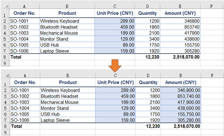
Clone and reuse a named style
When one set of formatting is needed in several places, registering it as a named style lets it be applied to any range by name, and a colour change has to be made in one place only. A named style lives on the workbook: create it with workbook.Styles.Add, set its properties, then apply it by name through Range.CellStyleName. The example builds a style of white text on a steel blue fill for the header row, then clones it and changes only the colours for the total line -- the change lands on the clone alone, and the original style is unaffected.
A named style is registered on the workbook and applied to a range by name:
| Syntax | Result |
|---|---|
workbook.Styles.Add('OrderHeader') |
Registers a named style called OrderHeader on the workbook |
headerStyle.Font.Color, headerStyle.Color, headerStyle.FillPattern |
Sets the text colour, the fill colour and the fill pattern one by one |
headerStyle.clone() |
Copies out a style of its own, with a number appended to the name |
sheet.Range.get('A1:E1').CellStyleName = headerStyle.Name |
Applies the named style to that range by name |
The steps are:
- Load the font file and the test data file into the VFS with
window.spire.FetchFileToVFS. - Create a workbook with
new Workbook(), load the input file withworkbook.LoadFromFile, and take the first worksheet withworkbook.Worksheets.get(0). - Create a named style with
workbook.Styles.Addand set its font name, size, bold, text colour, fill colour, fill pattern and horizontal alignment. - Apply the style to the header range by name with
sheet.Range.get('A1:E1').CellStyleName. - Clone it with the style's
clone(), change only the text colour and the fill colour, and get the variant the total line needs. - Apply the variant to the total line with
sheet.Range.get('A8:E8').CellStyleName. - Save the workbook with
workbook.SaveToFileand dispose of it withworkbook.Disposeto free resources.
The full code example below shows how to clone a named style and reuse it for different ranges in React:
function App() {
  const cloneNamedStyle = async () => {
    // get the Spire.XLS WASM module
    const xlsModule = window.wasmModule?.spirexls;

    // check that the module is ready
    if (!xlsModule) {
      alert('Spire.Xls is not ready yet');
      return;
    }

    // load the font and the test data file into the VFS
    await window.spire.FetchFileToVFS('ARIAL.TTF', '/Library/Fonts/', `${process.env.PUBLIC_URL}/font/`);
    const inputFileName = 'CopyCellStyle.xlsx';
    await window.spire.FetchFileToVFS(inputFileName, '', `${process.env.PUBLIC_URL}data/`);

    // load the workbook and take the first worksheet
    const workbook = new xlsModule.Workbook();
    workbook.LoadFromFile({ fileName: inputFileName });
    const sheet = workbook.Worksheets.get(0);

    // create a named style: white text on a steel blue fill, centred
    const headerStyle = workbook.Styles.Add('OrderHeader');
    headerStyle.Font.FontName = 'Arial';
    headerStyle.Font.Size = 11;
    headerStyle.Font.IsBold = true;
    headerStyle.Font.Color = xlsModule.Color.get_White();
    headerStyle.Color = xlsModule.Color.get_SteelBlue();
    headerStyle.FillPattern = xlsModule.ExcelPatternType.Solid;
    headerStyle.HorizontalAlignment = xlsModule.HorizontalAlignType.Center;

    // apply the named style to the header row
    sheet.Range.get('A1:E1').CellStyleName = headerStyle.Name;

    // clone it and change only the colours, giving the variant the total line needs
    const totalStyle = headerStyle.clone();
    totalStyle.Font.Color = xlsModule.Color.get_DarkBlue();
    totalStyle.Color = xlsModule.Color.get_LightYellow();

    // apply the cloned style to the total line
    sheet.Range.get('A8:E8').CellStyleName = totalStyle.Name;

    // save the workbook
    const outputFileName = 'CloneNamedStyle.xlsx';
    workbook.SaveToFile({ fileName: outputFileName, version: xlsModule.ExcelVersion.Version2016 });

    // dispose of the workbook to free resources
    workbook.Dispose();

    // read the result file from the VFS and start the download
    const fileArray = window.dotnetRuntime.Module.FS.readFile(outputFileName);
    const blob = new Blob([fileArray], { type: 'application/vnd.openxmlformats-officedocument.spreadsheetml.sheet' });
    const url = URL.createObjectURL(blob);
    const a = document.createElement('a');
    a.href = url;
    a.download = outputFileName;
    a.click();
    URL.revokeObjectURL(url);
  };

  return (
    <div style={{ textAlign: 'center', height: '300px' }}>
      <h1>Clone and Reuse a Named Style</h1>
      <button id="clone-named-style" onClick={cloneNamedStyle}>Clone and Reuse a Named Style</button>
    </div>
  );
}

export default App;
The worksheet after cloning a named style and reusing it:
FAQ
Copying the number format alone, without the fill or the border
Reason: A whole-cell copy takes the fill, font and border along with the number format, which is more than a change of display calls for.
Solution: Take NumberFormat from the source cell's style and assign that single property to the target cell's style, leaving the rest untouched:
// take the number format of the total line's quantity cell as the format to apply
const sourceStyle = sheet.Range.get('D8').Style;

// put only the number format onto the quantity column; the bold and the top border stay untouched
for (let row = 2; row <= 7; row++) {
  sheet.Range.get(`D${row}`).Style.NumberFormat = sourceStyle.NumberFormat;
}
Why a whole font object cannot be assigned to the target cell
Reason: Style.Font is a read-only property; it returns the font object the cell currently carries, so it cannot be replaced wholesale -- only the members hanging off it can be changed.
Solution: Set FontName, Size, Color, IsBold and the like one at a time. To bring the fill and the border across as well, assign the whole Style; to reuse a group of settings, register them as a named style and apply that style by name.
Does re-colouring a clone change the original style as well
Cause: clone() produces a copy that stands on its own, and once saved it takes a separate entry among the workbook's named styles; the name has a number appended to keep the two apart, so OrderHeader clones to OrderHeader1. Changing the text colour and the fill colour on the copy leaves the original where it was, still carrying the colours it had before the clone.
Solution: When several colour variants are needed, clone them all from the same base style and adjust each one separately; the definition of the base style never moves.
A named style or a plain Style assignment -- which one to use
Cause: Assigning a Style copies the source cell's current look onto the target cell in one go, which suits a one-off move; Range.CellStyleName applies a named style registered on the workbook, so a format used over and over is referred to by a single name in the code.
Solution: For a one-off move of the look, assign the whole Style; for a format reused in several places, build a named style with workbook.Styles.Add and apply it by name.
Get a Free License
Spire.XLS for JavaScript offers a 30-day full-featured free trial license with no functional limitations. Apply here to evaluate before purchasing.
